7 Display features

This section describes the displays that map3d generates and what they mean; for specific information on how to control map3d and the displays, see Section 8.

7.1 Multiple surfaces

The idea of map3d has always been to display multiple sets of data on multiple surfaces; the limitation has been how much flexibility to include in a single invocation of the program. This version of map3d, as opposed to previous versions, can now handle multiple windows each with multiple surfaces. Surfaces can be moved between windows (see Section 8.3.1) When map3d displays multiple surfaces, each can exist in its own full window with its own border and window title bar, or, map3d can build a single main window with multiple sub-windows inside the main window. The user can reposition and resize each of these sub-windows using the Alt(Meta) key and the left and middle mouse buttons respectively. To create this layout of main window and frameless sub-windows, use the -b (borderless windows) option when launching map3d as described in Section 4.3.

7.2 Surface display

The basic forms of display of the surfaces are

• nodes or points from each surface
• connectivity mesh
• shaded surfaces based on either the geometry or the associated scalar values, with a number of different rendering options.
• landmarks superimposed on the surface display

7.3 Mesh Rendering

Often the purpose of map3d is to render a geometry consisting of nodes and connectivities and there are several basic modes of rendering this information.

Points:

display just the nodes of the geometry as dots or marked with spheres.

Connectivities:

display the connectivity information for the mesh as lines joining the nodes.

Elements:

treat each polygon in the mesh as an element and render it in a way that shows its surface; for triangles, simple render each triangle surface; for tetrahedra there is no specific rendering in this version of map3d.

Elements and connectivities:

map3d also supports a hybrid mode of rendering that shows outward facing triangles (using the convention of counterclockwise ordering) as elements but backwards facing triangles as connectivities.

map3d also has the ability to render all elements with a lighting model. This is especially useful for displaying the elements of the mesh. Additional controls to note are depth cueing, which can reveal the depth relationships between elements of the mesh.

7.4 Surface Data Display

The main use of map3d is to display scalar data associated with geometry and there are numerous options and controls to facilitate this. The two basic ways of conveying scalar value information are as shaded surfaces and contour lines and map3d supports each separately, as well as in combination. For surface shading, there are several basic rendering modes:

Flat:

each triangle received a single color that depends on the mean value of the scalar value over that triangle.

Gouraud:

the colour of each triangle values linearly with the value at each of the vertices. The current version uses texture mapping to achieve more desirable results, but if your hardware does not support texture mapping, you can toggle it with the g-key.

Banded:

the regions between contour lines have a constant color, even if the contour lines are not visible.

Contours:

this can be a separate rendering mode, or combined with any of the three modes above. Contours are lines that trace iso-values over the surface of the geometry.

7.4.1 Data scaling

There is a wide variety of options available for mapping scalar values to colour and contour levels. One can picture the process as based on four facets:

Extrema:

the extrema of the data and the selected colour maps determine the basic parameters of how value maps to color. map3d maintains a detailed list of data extrema organized both by time signal, time instant and by surface. Thus it is possible to determine extrema based on just the most local of conditions--a particular frame and surface--or by more global conditions--the full range of frames or the full set of surfaces.

Scaling function:

the mapping between value and color occurs according to some mathematical function, the simplest of which is linear. The scaling function uses the selected extrema and describes a complete mapping between value and color.

Mapping:

by scale mapping, we mean how the translation from value to color treats positive and negative values. We may choose to map uniformly between the extrema or to apply different extrema or functions to the positive and negative values.

Color maps:

the color displayed for a particular scalar value depends on the actual range of colors and their order in the color map.

map3d can adjust all four facets of the scaling to create a wide range of displays. Note that all surfaces conform to the first three scaling options (there is only one scaling range, function, and mapping that corresponds to all surfaces). We also chose to limit some of these options, however, in an effort to create reproducible displays that reflect standard within the field. Of course, we chose our field, electrocardiography, as the basis, a fact for which we make no apologies and simply encourage others to make similar choices for their own field and implement map3d accordingly. Subsequent versions of map3d will support this flexibility.

Below are the specific choices that map3d offers to control data scaling and display

Scale range

map3d supports several selections of range over which to look for extrema. In local range, only the data presently visible are scanned for extrema--this is the default. In the full global range, all the data in the entire dataset are used, even those not presently visible on the display. In between these cases, one can have global in time and local in space, i.e., we scale each surface separately but use all time values for that surface. Or one can select local in time and global in space, in which map3d scans all surfaces for the data extrema, but for each time instant separately.

The user can also select group scaling, where he assigns surfaces to groups and the range is based on the group min/max (either local in time or global). Groups are assigned by the menu. The user can also do slave scaling, where he assigns one surface (slave) to another's (master) range. The slave surfaces are currently only set through the command line, by placing a -sl num (where num is the surface number of the master) after declaring the slave surface. See Section 8.2.3 and Section 4.4 for details.

If these options are not suitable, the user can select his own scaling scope for maximum and minimum values. This can be set via the command line (see -pl and -ph input parameters in Section 4). or in the Contour Spacing dialog (see Section 8.5.5). While the rest of the scaling range options are set once for all surfaces, whether or not an individual surface corresponds to the default range can be selected through the Contour Spacing dialog as well.

Scale function

The scale model describes the way in which scalar data are mapped to colours (or contours). The present choice is linear, but the next version of map3d will include: linear model, which simply maps the data to a range of colours in a completely linear fashion, i.e., $colour = K \phi$; the logarithmic model, which highlights the lower level data values at the cost of poorer resolution at the higher levels i.e., $colour = A\log(\phi) + B$; and the exponential model, which does the opposite, compressing the smaller levels and expanding the higher ones to span a wider colour range, i.e., $colour = A e^{B\phi}$.

The two schemes with fixed numbers of contours, log/7-levels and log/13-levels both map the upper decade ($\phi_{max}$ to $\phi_{max}/10.$) of the potential data range into a fixed set of logarithmically spaced values. These values are composed of a mantissa from the standard E6 (1.0, 1.5, 2.2, 3.3, 4.7, 6.8, and 10.) and E12 (1.0, 1.2, 1.5, 1.8, 2.2, 2.7, 3.3, 3.9, 4.7, 5.6, 6.8, 8.2, and 10.) number series, and an exponent such that the largest mantissa falls into the range 1.0 to 10. Hence as long as the extrema is known, it is possible to read absolute values from the individual contour lines.

Scale Mapping

There are several different ways to manage the way positive and negative data are treated in the scaling transformations in map3d. The current version supports the simplest, or true mapping, in which the data are used as they are with no consideration of positive or negative values--the color map spreads evenly across the range of the extrema. Subsequent versions will support the symmetric scale mapping, which sets the positive and negative extrema symmetrically--the larger (in the absolute value sense) determines both maximum and minimum data values. Also to appear in the net version is the separate scale mapping, in which the positive and negative extrema are treated completely separately--`half' the colours (and contours) are used for the positive values, half for the negative values. This is equivalent to producing maps with the same number of contours for both positive and negative values, even when the positive data have a different absolute maximum value than the negative data.

Colour Map

There are four different colour maps presently implemented with every chance of more to come. The user can select which colour map to use. The choices currently implemented are:

Jet map

(default) The Jet map is the same as the one used in MATLAB. Colours range from dark blue (for negative extrema) through greens (near zero) to dark red (positive extrema). Jet utilizes a minimal set of similar color, particularly of greens and yellows, a complaint of the Rainbow map.

Rainbow map

Colours range in rainbow fashion from blue (for negative extrema) through greens (near zero) to red (positive extrema).

Red (+) to Green (-)

Largest negative value is coloured bright green, dark grays are for the region near zero, and positive values appear red.

Black (+) to White(-)

Grey shades from black for small values to white for large ones.

Note that for each color map, the direction of the mapping to value can be inverted, e.g., in the default directions, blue indicates small or negative values and red indicates large or positive values. Inverted, this map uses red for small values and blue for large values.

Contours

Contours will be spaced according to the scaling parameters mentioned above. The number of contours or contour spacing can be changed in the Contour Dialog (See Section 8.5.5). If 'contour spacing' is selected, the spacing will determine the number of contours based on the range. If the function is linear and the mapping is true, the gap between contours will be the number specified in the dialog.

7.4.2 Scalar data reference

Related to scaling is the reference channel used for the displayed scalar data. By default, we assume that scalar values already have the right reference and we do nothing to change that. The user can, however, select a new reference and then subtract that reference from all signals in the surface. This is done by selecting the ``Reference lead - single value'' or ``Reference lead - mean value'' from the Picking menu (See Section 8.6). There are at present two types of references that map3d supports:

Mean as reference:

Selecting the mean as reference causes map3d to subtract the average value over each surface for each instant in time from the scalar data on that surface. Selecting the ``Reference lead - mean value'' from the Picking menu automatically does this, and can be undone by selecting ``Reset Reference'' from the same menu.

Selected lead as reference:

It is also possible to select a single channel of data and use that as the reference signal. This is done by first entering the the pick mode called ``Reference lead - single value'', and then selecting the reference node (See Section 8.2.1) performs this operation. The rest of the nodes then use that node as a reference value. Selecting a new reference lead works properly, i.e., the effect is not cumulative but first restores the data to the original state, than applies the new reference, and this can all be undone by selecting ``Reset Reference'' from the same menu.

7.5 Landmarks

Landmarks provide a means to include visual icons and markers in the surface display in map3d. They are not meant to render realistically but simply to be cues to assist the user in identifying perspective or features of the surfaces. The list of support landmarks reflects our current usage for bioelectric field data from the heart but many of the landmark types are general purpose and hence useful in other contexts.

Section 6.5 describes the currently support landmark types and the files that contain them. Display of each landmark type depends on the type and user controlled options (see Section 8 for details on controlling the display).

7.6 Clipping Planes

Clipping planes allow you to remove from view certain parts of the display so that you can better see what is left. So everything on one side of the clipping plane is visible and everything on the other is not.

We have two clipping planes in map3d and their position and alignments are adjustable as well as their relation to each other--we can lock the clipping planes together so they work like a data slicer, always showing a slice of constant thickness.

The controls for clipping planes are adjustable from the menus (see Section 8.2.3) and also via keyboard controls (see Section 8.2.2. The basic controls turn the two clipping planes on and off, lock them together, and lock their position relative to the objects in the surface display. By unlocking the last control, you can select that part of the display you want to clip; the default clipping planes are along the z-axis of the object (up and down). To control position of the planes along their normal direction, just keep hitting the bracket keys ([] and {}).

7.7 Background image

A background image may be useful in providing additional information. See the usage. If you want the image to line up in the geometry, you can specify geometry coordinates to force the image to line up with the geometry by specifying opposite coordinates of the geometry as parameters to the image. Note that the z in the (x,y,z) min and the (x,y,z) max should be the same.

7.8 Node marking

Node markings are just additional information added to the display of the nodes. This may be as simple as drawing spheres at the nodes to make them more visible, or as elaborate as marking each node with its associated scalar data value. Section 8.2.3 describes these options in detail.

7.9 Time signal display

Display option for the time signal are very modest in this version of map3d. This will change...

Figure 2: Time signal window layout. Vertical line indicates the frame currently displayed in the surface plot. Text annotations can vary with the data content and mode settings.

 

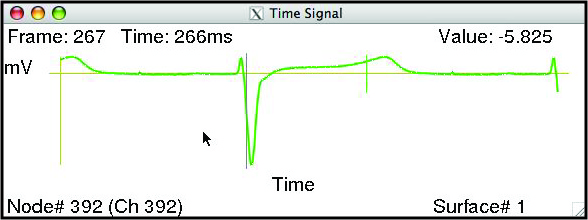Figure 2 shows the layout and labeling of the scalar window. Font sizes adjust with the window size and the type of units may be explicit if the time series data (.tsdf) files contain this information.

For directions on how to control the time signal window, see Section 8.4.