Next: 7 Display features Up: manual Previous: 5 Script Files Contents
In this section, we describe the contents and formats of all the input files that map3d uses to get geometry, data, and much more.
The input of geometric data for map3d occurs via files and we support three different formats at present. The simplest (and oldest) is a set of ASCII files that contain the points or nodes of the geometry--stored in a file with the extension .pts--and the connectivities that described polygonal links between nodes--stored as line segments (.seg files), triangles (.fac files), and tetrahedra (.tetra files). To satisfy a need for more comprehensive and compact storage of geometry information, we have developed a binary file format and created the graphicsio library to manage these files. Finally, in recognition of the ubiquity of MATLAB, as of version 6.1, there is support for reading .mat files, which have an internal structure that included node and connectivity information. Below, we describe each of these files and how map3d uses them.
The characteristics of a .pts file are as follows:
The characteristics of a .fac file are as follows:
At the CVRTI we have developed a binary file system for efficient storage of complex geometry and associated attributes, a part of what we call the graphicsio library. Extensive documentation of this format is available from Rob MacLeod (macleod@cvrti.utah.edu) (www.cvrti.utah.edu/~macleod/docs).
Briefly, each graphicsio geometry file contains one or more sets of node locations and, optionally, connectivities for polygonal elements composed from those nodes. It is possible in graphicsio files to associate scalar, vector, and tensor values to nodes or elements, the most relevant example of which are channel pointers, stored as a set of scalar values associated with the nodes of the geometry. Each graphicsio geometry file can contain any number of sets of geometries, each with different nodes and connectivities. A typical example for map3d would be a single .geom file that contains information from multiple surfaces that we might want to display together.
map3d is capable of reading surface geometry from either single surfaces or from all surfaces contained in a multi-surface geometry file. Command line arguments controls the selection, as we describe in the next section.
map3d can read .mat files generated by MATLAB as long as they are organized according to the following guidelines:
To prepare a structured .mat file is very simple, for example using the following commands:
     >> geom.pts = ptsarray;
     >> geom.fac = facarray;
     >> geom.channels = 100:164
     >> save mygeom.mat geom
where ptsarray is a facarray is a mygeom.mat is the name of the resulting .mat
file. The channels information indicates that there are 64 nodes in the
geometry and they expect to get time signals from channels 100-164 of a
data file. (See Section 6.4 for more information on
channels.
map3d can also read geometry from a landmark file (See Section 6.5 below), where you specify a series of connected points and radii. map3d will automatically connect and triangulate them, and will also associate scalar data with them. Note that currently there is no channels support for landmark geometry.
In map3d the -f option determines in which files the geometry is to be found. Starting from the filename that follows -f, which may or may not include a file extension, the program looks for all possible candidate geometry files and queries the user for resolution of any ambiguities. Thus, with the arguments map3d -f myfile, map3d3d looks for myfile.geom, myfile.mat, myfile.pts, myfile.fac, etc, and tries to resolve things so that a valid geometry description is found. It is possible to direct this process by typing the geometry filename with an extension according to the following rules:
| Extension | Effect |
| none | look for files with the extensions .pts, .fac, .tetra, and .geom and if an incompatible set are present (e.g., both .pts and .geom), ask user which to take |
| .pts | take only the .pts file and ignore any connectivity or .geom file |
| .fac | take .pts and .fac and ignore any .geom files present. |
| .geom | take the graphicsio geometry file and ignore any others present. |
| .mat | take the MATLAB file and ignore any others present. |
A further way to read geometry into map3d is to use the geometry filename that can be optionally contained within the time series file (see Section 6.3) that contains the potentials. This requires that the .tsdf file be created with the geometry filename included; adding this after the fact is difficult. Note that even if a geometry filename is found in the .tsdf file, it can be overridden by the geometry file name specified in the argument list of map3d.
There are three ways of storing scalar values (typically electric potential in our applications) so that map3d can recognize and read them. One is a simple ASCII file, one is a binary format developed at the CVRTI, and the third is MATLAB.
One way to package the scalar data values that are assigned to the points in the geometry is the .pot file. In the default condition, the scalar values in the .pot files are ordered in the same way as the node points in the geometry file with simple one-to-one assignment. With a channels file, it is possible to remap this assignment, as described in Section 6.4).
The rules for .pot files are:
One efficient and flexible way to store scalar values is by means of the time-series data file format developed at the CVRTI, also as part of the graphicsio library. Each time series data file (.tsdf files) holds an entire sequence, or time series of scalar data in a single file, along with some information about the contents, type, units, and global (i.e., that apply to all channels) temporal fiducials from the time series. For more details on this file format see www.cvrti.utah.edu/~macleod/docs/graphicsio.
Here are some concepts of the time series data file structure that are relevant to the different modes of operation described in this manual.
map3d -w -f geomfile.geom@1 -p datafile.tsdf -s 10 130 -i 2
specifies that surface 1 from the geometry file geomfile.geom
should be used to display frames 10 to 130, taking every second
frame, from run 2 of the time series data file datafile.tsdf.
There is an extension to the graphicsio library that defines a container file format for a set of time series data (.tsdf) files, and can contain parameters extracted from the associated time series. These files are actually small databases and we use a modified (patched actually) version of the GNU Database Library (GDBL) to manage them.
Examples of programs and libraries that provide support for .tsdfc files include Everett, a program by Ted Dustman for initial processing of mapping data, Matmap, a set of MATLAB uilities by Jeroen Stinstra with a similar functionality, and tsdflib (as yet undocumented), a library created by Ted Dustman, Rob MacLeod, Jenny Simpons, and Jeroen Stinstra that provides C-language access to container files.
For more information on container files, see the documentation for the graphicsio library at www.cvrti.utah.edu/~macleod/docs/graphicsio/.
You can also store and read scalar values in .mat files, as a structure
with a single field called ``.potvals'', that contains a ![]() array,
where
array,
where ![]() is the number of data channels and
is the number of data channels and ![]() is the number of time
instants. There are additional fields in the structure that mimic the
information available in the graphicsio .tsdf file so--the complete list is
as follows:
is the number of time
instants. There are additional fields in the structure that mimic the
information available in the graphicsio .tsdf file so--the complete list is
as follows:
Note that only the 'potvals' field is required. A matlab array may
be one instance of these fields, a cell or struct array of them, or
simply an ![]() array of data. To read a matlab file with many time
time series, specify the time series on the command line with the '@' symbol
(See Section 4.4) or specify the time series in the
file browser. It will be shown by the label specified in the matlab file.
array of data. To read a matlab file with many time
time series, specify the time series on the command line with the '@' symbol
(See Section 4.4) or specify the time series in the
file browser. It will be shown by the label specified in the matlab file.
The commands to make a suitable .mat file are very easy in MATLAB, for example, to load 128 channels of time signals with unit of millivolt from an array sockinfo in MATLAB to a file called mysockdata.mat
    >> sockdata.potvals   = sockinfo(1:128,:);
    >> sockdata.unit = 'mV'
    >> sockdata.lavel = 'A set of cool sock data'
    >> save mysockdata.mat sockdata
A fiducial can be input currently also in three ways: via a .tsdfc file, where the potential and fiducial values are stored together, via a .fids file, a simple ASCII file containing the values for each node, or by means of the MATLAB file that contains the time series data.
The fiducial information in a MATLAB time series data file is stored in a
array of structures called fids, where each element of the array represents
one set of fiducials. This way, for example, there can be a set of ![]() activation times, another set of
activation times, another set of ![]() recovery times, and a set of
recovery times, and a set of ![]() Q-onset times. Each element of the array is, in itself, a structure, so
that the set of fiducials contains enough information for map3d to do a
useful display.
Q-onset times. Each element of the array is, in itself, a structure, so
that the set of fiducials contains enough information for map3d to do a
useful display.
The legal elements of a fids structure are as follows:
Here is an example of creating the structures for some fiducials in MATLAB:
   matdata.potvals = potvals;
   matdata.unit = unit;
   matdata.label = label;
   matdata.fids(1).type = 10
   matdata.fids(1).value = fidvals(:,1);
   matdata.fids(2).type = 13;
   matdata.fids(2).value = fidvals(:,2);
   save (outfilename, 'matdata');
The first three lines set up the time series data, as we have seen above. The lines 4 and 5 create a set of fiducials of type 10 and loads the values into that part of the data structure. Lines 6 and 7 do the same thing for a second set of fiducials, which have type 13. The final line saves the contents of the structure into a file.
The type value for fiducials is important as map3d associates colors to fiducial types to provide consistent display. Moreover, each type has an associated text label that map3d uses in the interface. The list of current fiducial types and their numbers is as follows:
| Fiducial Types | |
| Number | Type |
| 0 | pon, pstart |
| 1 | poff, pend |
| 2 | qon, qrsstart, qrson |
| 3 | rpeak, qrspeak |
| 4 | soff, qrsend, qrsoff |
| 5 | stoff, tstart, ton |
| 6 | tpeak |
| 7 | toff |
| 8 | actplus |
| 9 | actminus |
| 10 | act |
| 11 | recplus |
| 12 | recminus |
| 13 | rec |
| 14 | ref, reference |
| 15 | jpt, jpoint |
| 16 | baseline |
| 30 | pacing |
The characteristics of a .fids file are as follows:
    Example:
    1
    1 -1
    256 activation recovery
    1 8 212
    2 16 225
    3 9 214
    ...
    255 39 248
    256 25 237
Channels and leadlinks files, and the arrays they
contain, are identical in structure, but they have important functional differences. A run of map3d may require both, either, or
neither of these, depending on the structure of the data files and
geometries. The basic function of both channels and leadlinks information
is to offer linkages between nodes in the geometry and the data that is to
be associated with those nodes. The first file type, the channels file,
links the nodes in the geometry to specific time signals in a data file;
without channel mapping, the only possible assumption is that each node ![]() in the geometry corresponds to the same time signal
in the geometry corresponds to the same time signal ![]() in the data file.
Any other linkage of geometry and data channel requires there to be channel
information, typically either from a separate .channels file or stored with
the binary .geom file as an associated scalar value for each node.
in the data file.
Any other linkage of geometry and data channel requires there to be channel
information, typically either from a separate .channels file or stored with
the binary .geom file as an associated scalar value for each node.
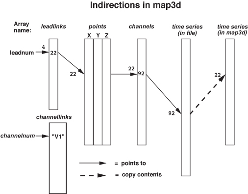 |
Leadlinks are purely for visualization and describe the connection between ``leads'', a measurement concept, with ``nodes'', a geometric location in space. In electrocardiography, for example, a lead is the algebraic difference between two measured potentials, one of which is the reference; ``unipolar'' leads have a reference composed of the sum of the limb electrode potentials. It is often useful to mark the locations of these leads on the geometry, which often contains many more nodes than there are leads. The most frequent use to date has been to mark the locations of the standard precordial ECG leads within the context of high resolution body surface mapping that uses from 32-192 electrodes. Another common application is to mark subsets of a geometry that correspond to measurement sites (values at the remaining nodes are typically the product of interpolation). In summary, leadlinks allow map3d to mark specific nodes that may have special meaning to the observer.
Figure 1 shows an example of lead and channels information and their effect on map3d. See the figure caption for details.
map3d handles this information in the following manner:
Note that map3d uses the channels arrays when loading scalar data into the internal storage arrays! Hence, the action of the channel mapping is not reversible. Should geometry nodes and data channels match one-to-one, there is no need for a channels array. It is also possible to define via a channels array the situation in which a single data channel belongs to two (or more) nodes in the geometry. The most frequent example of this occurs when three-dimensional geometries are ``unwrapped'' into surfaces in which what was a single edge is split and thus present at both ends of the surface.
In the leadlinks array each entry refers, by its location in the
array, to a particular lead #; the value at that location in the
array gives the number of the node in the geometry file to be
associated with this lead. For example if lead 4 has a leadlinks
entry of 22 (
![]() ), then map3d will display
node 22 in the geometry as ``4'', not ``22'' whenever node marking
with leads is selected).
), then map3d will display
node 22 in the geometry as ``4'', not ``22'' whenever node marking
with leads is selected).
Hence we have the situation of a node number ![]() in the geometry
displaying time signals from channel
in the geometry
displaying time signals from channel ![]() in the scalar data, but
labeled with string ``XXX''.
in the scalar data, but
labeled with string ``XXX''.
The sources of channels, leadlinks, and channellinks information are files, or parts of files, as outlined in the following paragraphs.
Information for the channels array is stored as an associated scalar with the information in the standard .geom files. At present, there is no leadlinks array stored in the .geom file but this could change in the future.
MATLAB geometry files can also contain an channels array is stored as a .channels field in the structure. See Section 6.1.4 for more details.
A .leadlinks file is an ASCII file, the first record of which
contains a line nnn leads, where nnn is the number of leads to
be described in the file (and also one less than the total number of lines
in the file). Each following record contains two integer values:
    32 Leads
    1   1
    2   42
    4   31
    7   65
    .   .
    .   .
    .   .
    32  11     <---- 32nd entry in the file, at line 33 of the file.
indicates that there are 32 leads to be linked (the geometry can, often
does, contain more than 32 nodes), and that lead #1 is called lead ``1''
and is node 1 in the geometry file. Lead #2 is at node 42, lead #3 is
called ``4'' and is found at node 31. Likewise, lead #4 is called ``7'',
and is located at node 65, and so on, up to lead #32, called ``32'', at
node 11.
Nodes listed in a leadlinks file that is passed to map3d with the -ll option can be marked in a number of ways, described more fully in Table 10 in Section 8.2.3.
A channels file is an ASCII file, the first record of which contain a
line nnn nodes, where nnn is the number of nodes to be
described in the file (and also one less than the total number of lines in
the file). There is one line in the file for each node of the geometry to
which we wish to associate scalar data. Each following record contains
two integer values:
For example, the file for a surface which reads:
    352 Nodes
    1    123
    2    632
    .    .
    .    .
    22   -1
    23   432
    .    .
    .    .
    352  12
indicates that there are 352 leads to be linked, and that the data value
for the first node is located at location 123 of the data file. For node
2, the data value is to be found at location 632, and so on. Node 22 does
not have any scalar data associated with it.
To see how map3d can display the node and lead information, see Sections 7.8 and 8.
Landmark files contain information for visual cues or landmarks that map3d can draw over the surfaces in order to aid and orient the viewer. Initial use was primarily for coronary arteries, but the idea has expanded to incorporate a number of different orientation landmarks. The original coronary artery class of landmarks requires only that each can be described as a series of connected points, with a radius defined for each point. The coronary landmark is then displayed as a faceted ``pipe'' linearly connecting the points at the centre, with a radius, also linearly interpolated between points, determining the size of the pipe. The landmark file can contain numerous, individual segments of such pipe-work, each of which is drawn separately.
Other classes of landmarks are described below, but all of them can be described in a file with the following general format:
| Line number | Contents | Comments |
| 1 | nsegs | number of landmark segments in the file |
| 2 | 1 type nsegpts [segindex] [segcolor] | segment number (1), type, number of points, with optional index number and color (color is a RGB triple, 0-255 each) |
| 3 | X, Y, Z, radius [label] | point location and radius of point 1, with optional label to be drawn at the point |
| 4 | X, Y, Z, radius [label] | point location and radius of point 2 |
| . | . | . |
| . | . | . |
| nsegpts + 2 | X, Y, Z, radius | point location and radius of last point in segment 1 |
| . | 2 type nsegpts [segindex] [segcolor] | segment number (2), type, number of points, with optional index number and color |
| . | X, Y, Z, radius [label] | point location and radius of point 1 |
| . | X, Y, Z, radius [label] | point location and radius of point 2 |
| . | . | . |
| . | . | . |
| . | X, Y, Z, radius [label] | point location and radius of last point in segment 2 |
| . | . | . |
| . | . | . |
| . | . | . |
| . | . | . |
The landmark types defined to date are the following:
| Name | Graph. object | Description |
| Artery | faceted pipe | a coronary artery/vein segment |
| Occlusion | coloured sphere | an experimental occlusion that could be open and closed |
| Closure | coloured sphere | a permanent occlusion that cannot be opened |
| Stimulus | coloured sphere | a stimulus site |
| Lead | coloured sphere | a particular electrode or lead location |
| Plane | rectangular parallolopiped | a visible (but not functional) cutting plane through the geometry (Note: do not confuse this with the cutting planes that map3d provides for slicing through the geometry). |
| Rod | lines | rod inserted into needle track to digitize needle electrode locations. |
| PaceNeedle | sphere | location of a pacing needle entry point |
| Cath | faceted pipe | location of catheter in a vessel |
| Fiber | arrow | local fiber direction indicator |
| RecNeedle | sphere | location of recording needle entry point |
| Cannula | tube | coronary vessel cannulus |
Specifying snare, closure, and stimulus requires a single point in the landmarks file, and the resulting sphere is coloured according to a set of values defined in the drawsurflmarks.c routine. At present, the values used are:
| Occlusion | cyan |
| Closure | blue |
| Stimulus | yellow |
and they are adjustable by the user, either via the Landmark menu, or by specifying a color for the segment
To specify a plane landmark requires three ``points''
| Point | X,Y,Z | Radius |
| 1 | First point of plane | Radius of the plane |
| 2 | Second point of plane | Thickness of the plane |
| 3 | Third point of plane | not used |
Rob Macleod 2007-03-01