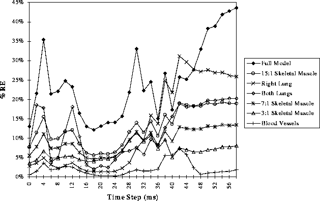
Figure 6: Values of RE between BSPMs computed with the homogeneous torso and those computed using the torso with the addition of the listed inhomogeneity as a function of time through the 60 ms of the QRS of a single beat.
While all three measures, ERMS, RE, and CC, were calculated for each pair of maps, the values for ERMS and RE responded identically to changes in inhomogeneities. Hence, we include only plots of RE and CC. The calculated ERMS, RE and CC values for all the simulations can be found on the World Wide Web at http://www.cs.utah.edu/~rklepfer/inhomogstudy.html. Note that the actual values of RE depend on the value chosen for the homogeneous isotropic conductivity.

Figure 6: Values of RE between BSPMs computed with the homogeneous torso and those computed using the torso with the addition of the listed inhomogeneity as a function of time through the 60 ms of the QRS of a single beat.
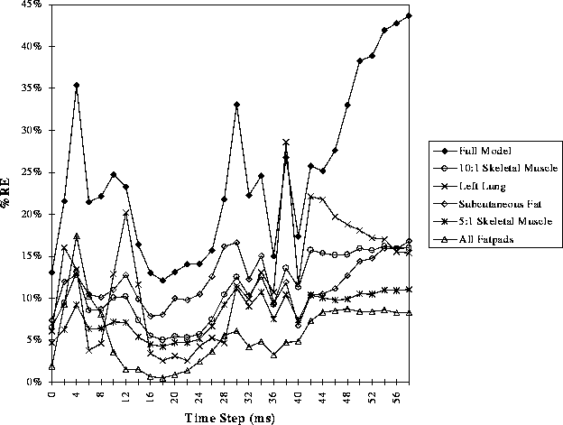
Figure 7: Values of RE between BSPMs computed with the homogeneous torso and those computed using the torso with the addition of the listed inhomogeneity as a function of time through the QRS.
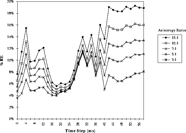
Figure 8: The RE values comparing BSPMs from the homogenous torso to those generated using a range of muscle anisotropy values in the torso model. Note the change in vertical axis scaling compared to previous plots.
Figures 6 and 7 show the RE for simulations in which a single inhomogeneity was added to the otherwise homogeneous isotropic torso. The data has been split into two figures to improve readability. The RE values for the fully detailed model are also included in both for comparison. The changes produced by including two of the inhomogeneities--the isotropic skeletal muscle and bone--were too small to include in the figures.
Figures 6 and 7 include examples of a finding seen throughout the studies; the relative error induced by many inhomgeneities depended strongly on the time instant, and, hence, on the potential distribution at each time instant. For example, the RE values for the right lung were among the smallest in both figures for the early part of the beat, but then increased to the first or second largest amplitude by the latter 15 ms of the QRS.
Another finding from Figures 6 and 7 is that the inhomogeneities of the more anisotropic skeletal muscle and the lungs generally had more influence on model error than the other inhomogeneities. This was most consistently the case late in the QRS. During early QRS, the error values for lungs tended to be smaller than, for example, those from the subcutaneous fat or skeletal muscle at lower anisotropy ratios.
Five different skeletal muscle anisotropy ratios were tested. Figure 8 shows the RE values for the different ratios. The notable finding here is that the level of error produced increased monotonically with the degree of anisotropy.
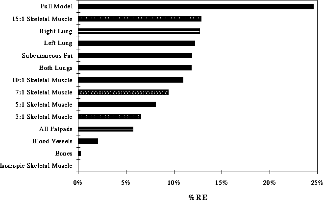
Figure 9: Average RE values across all time steps between the BSPMs for the inhomogeneity listed and those from the homogeneous case.
Figure 9 shows a compressed version of the information in Figures 6 and 7 - the average RE computed across all time instances between the homogeneous torso and those with the single inhomogeneities listed. They are ordered according to size of effect and thus represent a mean ranking of the effects of different inhomogeneities.
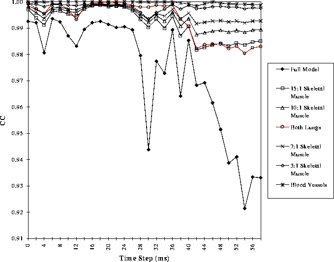
Figure 10: The correlation coefficients between BSPMs of the homogeneous torso and the those from the torso with the listed additional inhomogeneity as a function of time.
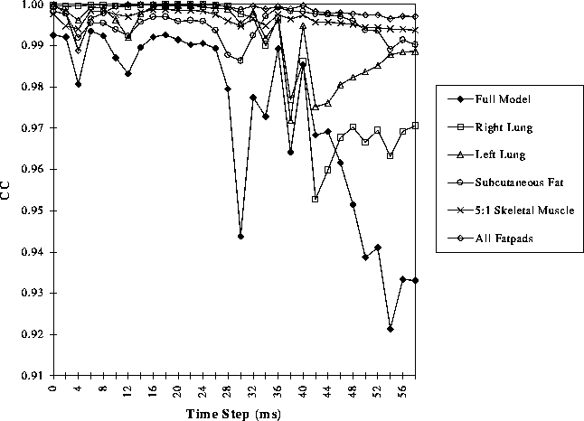
Figure 11: The correlation coefficients between BSPMs of the homogeneous torso and the those from the torso with the listed additional inhomogeneity as a function of time.
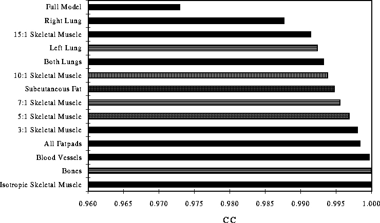
Figure 12: Average correlation coefficient across all time steps between the BSPMs for the inhomogeneity listed and those computed from the homogeneous case.
Figure 10 and 11 show the CC values for the same simulations from which Figures 6, 7, and 9 were derived. Just as for the relative error results, data for isotropic skeletal muscle and for bones were not included and the curves were split into two plots to improve readability. A comparison of RE and CC results reveals that the changes that occured by adding single inhomogeneities were more evident in the relative error than in the correlation coefficient.
Figure 12 summarizes Figures 10 and 11 into a single value for each inhomogeneity--the average CC across all time instances. The inhomogeneities are listed in descending order of their effects and we see that the ranking is almost the same as that in Figure 9. The two exceptions are that the right lung is switched with the 15:1 skeletal muscle and the subcutaneous fat dropped below the 10:1 skeletal muscle for the correlation coefficient data. Again, the findings of the RE data are reiterated here: the anisotropic skeletal muscle with larger longitudinal-to-radial fiber ratios and the lungs showed the larger effects.
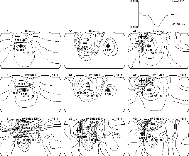
Figure 13: Computed BSPMs under different conductivity assumptions. Layout of the maps is identical to that in Figure 5. The rows of maps differ in the conductivities assumed with the homogenous torso used to generate the results shown in the uppermost row, the 15:1 skeletal muscle added to the homogeneous model in the middle row and their difference displayed in the lowest row.
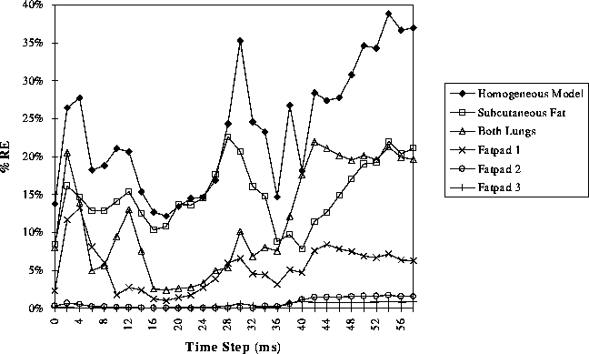
Figure 14: Values of RE between BSPMs computed using the full inhomogeneous model compared to those computed when each of the listed inhomgeneous regions was ``removed'', i.e., given the same conductivity value as the homogeneous torso model.
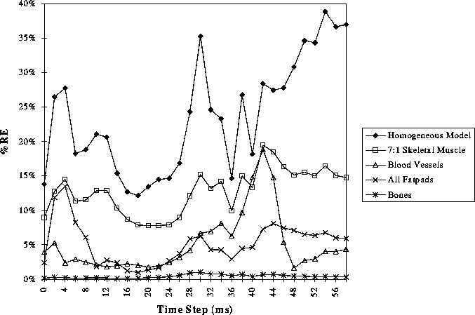
Figure 15: Values of RE between BSPMs computed using the full inhomogeneous model compared to those computed when each of the listed inhomgeneous regions was ``removed''.
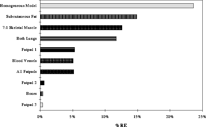
Figure 16: Average RE values across all time steps between BSPMs of the full model and the those using the full model with the listed inhomogeneity removed.
Figure 13 shows qualitatively the effects of including 15:1 skeletal muscle on the BSPMs of the model. The top row of the figure shows BSPMs generated from the homogeneous model; the BSPMs in the middle row were computed with 15:1 skeletal muscle included in the model. The bottom row shows the difference maps generated by subtracting the skeletal muscle map from the homogeneous map. The number in the upper left corner of each map is the time instant the map represents. The influence of the anisotropic skeletal muscle can be seen in the tendency for the isocontours of the skeletal muscle maps to be slightly more horizontal than the corresponding homogeneous model maps, a possible effect of the circumferential implementation of the skeletal muscle anisotropy.
The second set of simulations considered the difference between BSPMs of the full inhomogeneous model and the same model with one inhomogeneity removed. Figures 14 and 15 show the RE values calculated at each time instant for each of the inhomogeneities listed. The data for the homogeneous model is included in both figures for reference. The symmetry of the two types of simulations performed dictates that the difference between the homogeneous model and that with all inhomogeneities include, as shown in the first set of results, must be identical to the difference between the fully inhomogeneous model and that with all inhomogeneities removed, as shown in the second set of simulations. While comparison of, for example, Figures 6 and 14 suggests otherwise, the discrepancy lies only in the nature of the relative error calculation in which a different reference dataset was chosen based on the perspective. The correlation coefficient results presented below do not suffer from this bias and demonstrate identical results in both comparisons.
Figure 16 shows the average RE computed across all time instances between the fully inhomogeneous model and the full model with the inhomogeneity listed removed.
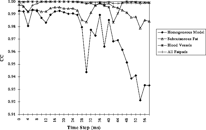
Figure 17: The correlation coefficients as a function of time between BSPMs of the full model and those of the model with the single inhomogeneity listed removed.
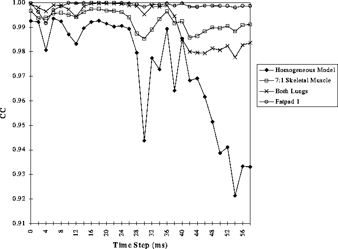
Figure 18: The correlation coefficients as a function of time between BSPMs of the full model and those of the model with the single inhomogeneity listed removed.
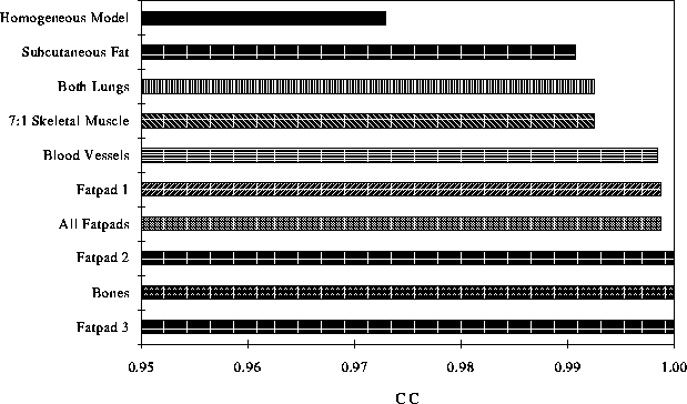
Figure 19: Average correlation coefficient across all time steps between BSPMs of the full model and those from the model with the listed inhomogeneity removed.
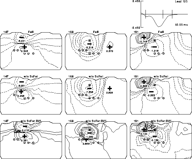
Figure 20: Computed BSPMs under different conductivity assumptions. Layout of the maps is identical to that in Figure 5. The rows of maps differ in the conductivities assumed with the full inhomogenous torso used to generate the results shown in the uppermost row, the full torso without subcutaneous fat in the middle row and their difference displayed in the lowest row.
Figures 17 and 18 show the CC calculated for each inhomogeneity at each time step and Figure 19 shows the averages for each inhomogeneity across all time steps. Figure 20 demonstrates the differences between BSPMs in the second set of simulations qualitatively. The top row shows BSPMs of the full model; the middle row shows the maps of the full model without subcutaneous fat. The bottom row shows the difference between these two maps at each time instant.