 |
Rob MacLeod and Brian Birchler
The goal of the lab is to develop some understanding of the biophysical basis and practice of electrocardiographic measurements. A secondary purpose is to examine the hypothesis that a current dipole is a suitable source model for the electrical activity of the heart.
The text book background for this lab is particularly weak so please consult the class notes and some of the web links from the class web site. Some particularly useful links are:
Note that the term ``lead'' here means the potential difference measured between two electrodes. Thus, each single lead requires two electrodes. We talked in class about bipolar versus unipolar leads and this lab will illustrate their meaning and differences.
Please perform the Limb Leads, Frank Lead ECG, and Standard ECG exercises (described below) in your usual groups of 2 and 3 students. Use the same subject for all parts.
Equipment for performing the Body Surface Mapping (BSPM) may not be available; if not, you will receive a point to data to be analyzed for your lab report. Groups of 6 students at a time should consult with Dr. MacLeod at some point during the lab for a tutorial of map3d, the program necessary for visualization and analysis of the BSPM data.
The limb leads are part of the legacy of Wilhems Einthoven, developer of
the string galvanometer and winner of the 1926 Nobel Prize for his advances
in electrocardiography. The idea was based on the current dipole as a
source of cardiac electrical activity. The goal of the leads developed by
Einthoven was to capture the projection of the cardiac dipole in the
frontal plane based on an equilateral triangle coordinate system. The
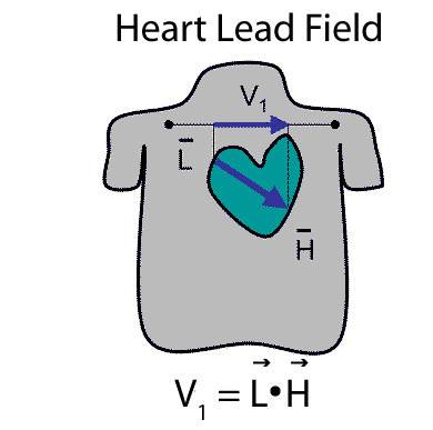
underlying formalism of the limb lead system (and the Frank lead system developed
later) is the lead field, a function that projects a current dipole
source to any point on the body surface as shown in
Figure 1. The lead field vector
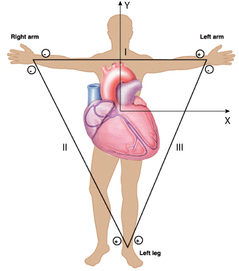
In this lab, you will record the standard limb leads in sequence, according
to the diagram in Figure 2. Note the polarity of the
leads-this is important to check when performing the measurements. An
inverted lead (i.e., with the connections reversed) will result in useless
data during the analysis. Note also that the limb leads are based on an
equilateral triangular coordinate system and that it will be necessary to
transform them to a Cartesian system to compare with the other lead systems
we will investigate. HINT: This requires more than just taking the sin/cos of the vectors.
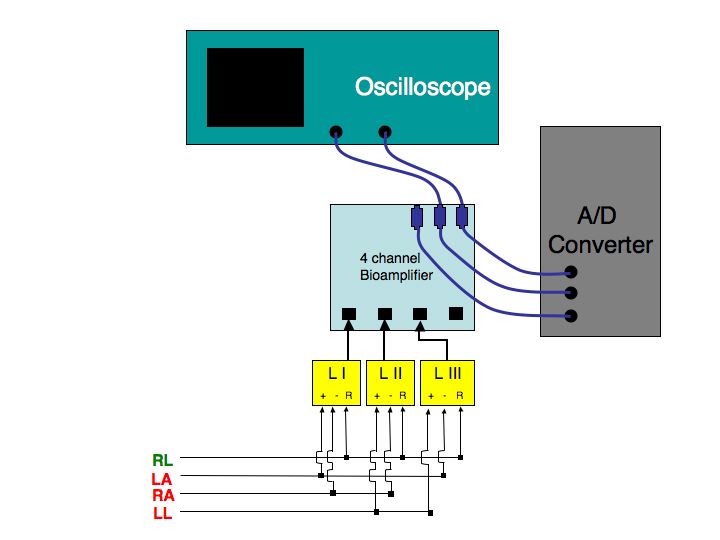
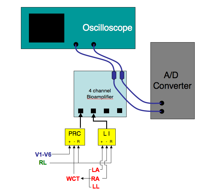
The circuit diagram for the associated measurements in the lab is shown in
Figure 3. Note here again the importance of getting
proper polarity of the leads. Don't trust the diagram but check yourself
to make sure the connections make sense. Failure to check this during the
measurements will result in data that cannot be corrected later!
The steps in setting up this basic ECG measurement are illustrated in
Figure 3 and are as follows:
Now ensure that you have a good signal on the oscilloscope and make
adjustments as necessary. Here, perhaps more than in other labs,
it is worth the time to achieve the best quality signals possible.
Try and move wires around, have the subject sit very quietly and make sure
to prepare the skin fully as these all contribute to high quality
recordings. Once you are satisfied with the signal quality, carry out the
following steps:
After the lab, follow the instructions in Section 3 below to
compute the dipole direction from the limb lead signals.
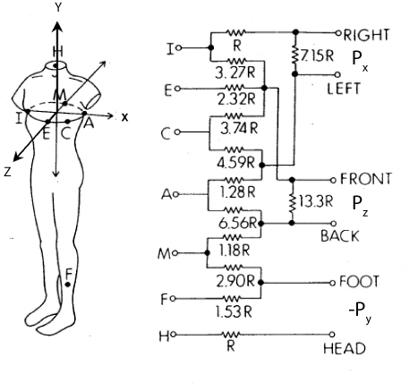
The goal for the Frank electrode system is to capture the three-dimensional
extent of the heart dipole. For this, it is necessary to measure potential
differences not just in the frontal plane, as in the limb leads, but along
the antero-posterior (front-to-back) axis of the body. The diagram in
Figure 5 illustrates the original Frank lead system
[1] and we will use a simplified version of this.
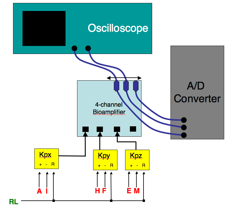
The circuit diagram for the associated measurements in the lab is shown in
Figure 6. Again, be very careful about lead polarity and
lead placement in these measurements. Note that you can capture all three
leads at once on the A/D converter but must select two leads to display on
the oscilloscope. HINT: CB8ChanScope cannot record just 3 channels and
crosstalk occurs on empty channels. This does not affect your recorded
signals but may be confusing. I suggest connecting channel 4 to ground.
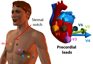
The standard 12-lead ECG lead system seeks to increase sensitivity to local
activity and so places the leads on the chest close to the heart, as
Figure 7 indicates. The source assumptions for this
lead system are not of a current dipole but rather each lead is
thought to reflect the electrical activity of a nearby region of the heart.
The circuit diagram for the associated measurements in the lab is shown in
Figure 8.
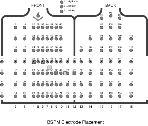
The goal of body surface mapping is to record the entire distribution of
electric potential over the surface of the torso and thus to create an
image of this field rather than a small number of time samples. To this
end, such systems measure at from 32-200 sites on the front (and sometimes
back) of the torso. Figure 9 shows an example of a
BSPM system with 120 electrodes attached to both the front and back of the
torso.
The BSPM system used in the lab is based on 32 leads attached to the
anterior surface of the torso. To select these 32 sites, investigators
recorded a database of maps at much higher resolution and then extracted
from them the most meaningful leads [2,3] according to
a statistical estimation strategy. To create maps of potential
distribution from the 32 leads requires a post processing step that applies
this estimation, in the form of a matrix. The resulting maps contain 192
leads. We will use a program called map3d to display these data.
See Appendix A below for details of the estimation
scheme. The data posted to the web site is already appropriately
transformed and is ready for use.
There are a set of steps to perform on the recorded signals before they are
available for analysis. With the processed data it will then be possible
to determine the direction of the heart dipole using each of the lead
systems.
For this lab, identify for each beat in your recording two points, one
before the PQRST and one after it, and use those to fit a straight
line. Then subtract this line from the entire beat. The MATLAB
function POLYFIT provides a simple means of fitting a segment of the
signal to a straight line (or any other higher order polynomial as
well).
Note that because of the redundancy in the system, you will only need
two of the limb leads to determine the heart vector; pick any two (but
be smart, i.e., use lead I). Include a diagram and the steps of
your derivation with the report
HINT: LII is NOT H and Hy
The Frank lead system provides directly the three orthogonal leads of the
dipole vector so that no calculations are necessary. To compare with the
results of the limb leads, plot the same values as described for the limb
lead case in the frontal plane (x - y
Make sure to apply the same type of baseline correction as for the
limbs leads and divide the signals into QRS and ST complexes, then create
separate loops for each of these two parts of the ECG.
The notion of the dipole vector is not so well integrated into the
electrocardiography of the precordial leads (standard ECG). As
Figure 7 shows, each lead represents a vector direction
based on a line from the body central axis through the electrode location
on the body surface.
BSPM captures all the potentials on the body surface and the analysis of
such maps occurs not in terms of dipoles but by the distribution. We will
take a similar course in analyzing some pre-recorded BSPM data from a
previous lab. We will include in the next lab a demo of the BSPM method
but in the meantime, please proceed as follows:
There is a single set of four mapping data files, one for each of
positions we had Andrew (a student in a previous class) take. Download
all these files. Each file is in MATLAB format as a data structure
with three items, the time signals, called ``potvals'', the units,
called ``unit'', and a text label, called ``label''.
For example, to read in the file andrew-sitting.mat and see
its contents in MATLAB:
Use the standard lab format for this one:
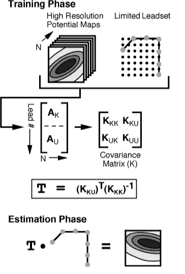
Here are the details of the estimation, provided only for the curious.
The first component of the estimation technique is the training phase,
which begins by defining the training database and selecting the particular
leadset. The training database is composed of N
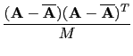
The next step in the training phase is to calculate the covariance matrix
The result from the training phase is an
MU x MK
This document was generated using the
LaTeX2HTML translator Version 2008 (1.71)
Copyright © 1993, 1994, 1995, 1996,
Nikos Drakos,
Computer Based Learning Unit, University of Leeds.
The command line arguments were:
The translation was initiated by Rob Macleod on 2011-03-02![]()
![]()
2.2.0.1 Lead placement
Note also that rather than the classic limb
leads based on electrodes attached to the arms and legs, we will use an
equivalent system based on electrode sites on the thorax. This
modification makes the lead placement slightly easier but the main
advantages are practical in that electrode wires are shorter (less noise)
and easier to manage, both in the lab and in clinical practice.
2.2.1 Lab steps
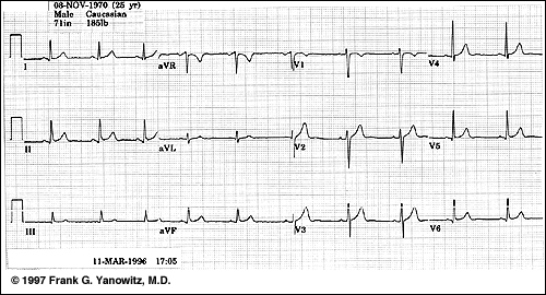
You can check that you have proper polarity by comparing the measured
signals to the sample in Figure 4 below.
2.3 Frank Lead ECG
2.3.1 Lab steps
2.4 Standard ECG
2.4.1 Lab steps
![]()
2.5 Body Surface Potential Mapping (BSPM)
3 Post Processing
3.1 Limb leads
![]()
![]()
![]()
3.2 Frank leads
3.3 Precordial leads
3.4 BSPM
www.cvrti.utah.edu/~macleod/bioen/be6000/labnotes/ecg/data
and then (right-click or control-click on the files you want to
download and then select ``download link to disk'' or equivalent
      >> load 'andrew-sitting'
      >> whos
        Name       Size                    Bytes  Class

        run2       1x1                   2032584  struct array

      Grand total is 254061 elements using 2032584 bytes

      >> run2

      run2 =

          potvals: [192x1323 double]
             unit: 'uV'
            label: 'SITTINGUPANDREW/    24-FEB-05/G=6/      '
In this case, ``run2'' is the name I gave to the data when I created
andrew-sitting.mat so you will see a different name for each
of the files. This file contains 192 channels of data with 1323 time
instants in each of those channels. To access the time series data,
use the notation run2.potvals and treat this as the matrix
name. Each row in run2.potvals is a time signal for a
particular channel. So to plot channel 47 of the data, use the MATLAB
command
>> plot(run2.potvals(47,:))
Generate these leads and then find the direction of the vector loop
at its maximum and compare the direction and magnitude for each of
the positions of the subject, i.e., laying flat, on the left side,
on the right side, and sitting. The question to answer
here is whether a change in body position is enough to cause a
discernible shift in the vector direction.
4 Lab report
A. Estimation process
![]()
![]()
![]()
![]()
![]()
![]()
![]() where
where
![]() =
=  ,
,
(1) ![]()
![]() where
where
![]()

![]() ,
,
(2) ![]()
![]()
![]()
![]()
![]()
![]() = (
= (![]() )T (
)T (![]() )-1.
)-1.
(3) ![]() where AKi
where AKi
AUi =
![]() x AKi,
x AKi,
(4)
Bibliography
An accurate, clinically practical system for spatial
vectorcardiography.
Circ., 1:737-749, 1956.
Limited lead selection for estimation of body surface potential maps
in electrocardiography.
IEEE Trans Biomed. Eng., 25:270-276, 1978.
Clinically practical lead systems for improved electrocardiography:
Comparison with precordial grids and conventional lead systems.
Circ., 59:356-363, February 1979.
About this document ...
ECG Measurement and Analysis
Copyright © 1997, 1998, 1999,
Ross Moore,
Mathematics Department, Macquarie University, Sydney.
latex2html -split 3 -no_white -link 3 -no_navigation -no_math -html_version 3.2,math -show_section_numbers -local_icons descrip
Rob Macleod
2011-03-02