Dissection and Contraction of Frog Heart
Rob MacLeod and Alex Brownell (aabrownell@yahoo.com)
To examine the anatomy and basic contractile physiology of the frog heart.
This lab provides background information for the subsequent study of the
physiological response of the frog heart to external stimuli, which we will
cover in the next lab session.
There are a number of excellent web sites you can peruse to find background
information relevant to this lab. We will cover some basics in class, but
please at least go through the virtual dissection site at
curry.edschool.virginia.edu/go/frog/Frog1/menu.html.
The full list of web sites to visit include:
We assume you have a working knowledge of MATLAB. If this is not the case,
please let me know and the TA for the lab, Alex Brownell (aabrownell@yahoo.com), will give a
tutorial on Matlab. For more information, you can go to the web sites
listed at
www.cvrti.utah.edu/~macleod/software/matlab-info.html
and consult
any of the enormous number of books written about Matlab.
2.1 Materials
The equipment required consists of:
- Digital camera to take photos of the frog during dissection
- Dissection pan with 4 needles
- Dissection kit you used in the anatomy experiment.
- Two bioamplifiers
- Force transducer
- 2 magnetic clamp stands
- Bipolar electrode
- Oscilloscope
- Computer with acquisition program (
C:\\bioen\CB8ChScope)
- 20 ml vials for drug samples
- Plastic eye-droppers
- suture needle with thread attached
- Batteries for the force transducer
- medium sized vial containing Ringer's solution,
composed of:
- NaCl: 200 ml (stock 4M),
- KCl: 20 ml (stock 1M),
-
MgCl2
: 20 ml (stock 1M),
-
CaCl2
: 4 ml (stock 1 M),
- NaOH: 25.8 ml (stock 1 M)
- D-Glucose: 1.8 g,
- Hepes: 11.44 ml (stock 1 M),
- pH: 7.4,
- De-ionized water: to make 2 L,
- Total Volume: 2 L.
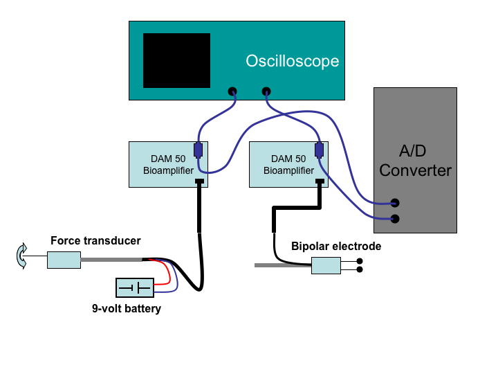
Figure 1:
Circuit diagram for the recording of
contraction and electrograms from the frog heart.
 |
Please carry out the following steps (Note Do not start the frog
dissection until you have completed all the setup steps!):
- Setting up the measurement circuit according to
Figure 1:
- Connect the battery to the pressure transducer and hook up
the wires from it to the input of one of the bioamplifiers.
- Place a T-connector on the output of the bioamplifier and
then connect one end to the input of the oscilloscope and
the other to the inputs for the computer A/D converter.
Use channel one for both the oscilloscope and A/D converter.
- Adjust the settings on the bioamplifier to get a clean signal
on the oscilloscope in which you can see the response to
gentle bending of the force transducer. Start with the
following settings on the bioamplifier:
- DC coupling
- Low filter at lowest frequency setting
- High filter at low to moderate frequency
- Gain at or near maximum
On the oscilloscope, try the following settings (make sure
all settings are in calibrated mode, i.e., latched into fixed
settings):
- DC coupling
- 1 Volt/div
 0.5 s/div
- Launch the acquisition program (
C:\bioen\CB8ChanScop)
computers for acquiring the signals. Then select sampling
parameters from the program (sampling rate of 100-200 is adequate)
and run it to make sure it acquires signal.
Figure 2:
Calibration of the force transducer.
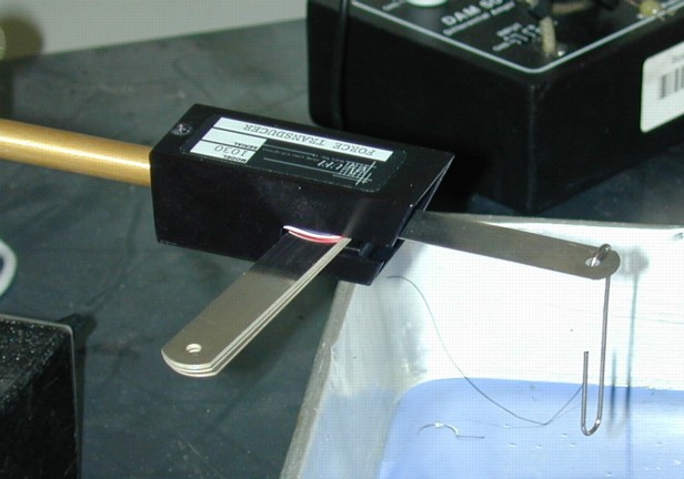 |
- Calibration of the force transducer:
- Mount the transducer in the magnetic stand and make sure only
the thinnest blade is aligned with the transducer handle (all the
other blades should be perpendicular to the handle), as shown in
Figure 2. Rotate the transducer so the flat
side of the blade is parallel (horizontal) to the table;
deflections in the up and down directions should cause the signal
on the oscilloscope to change.
- Use a small Phillips screwdriver to remove the screw and
slide the cover out of the way. Put the cover and the screw
carefully aside for later re-attachment.
- Use a small straight screwdriver to adjust the zero of the
transducer. This can be a little tedious as many turns of the
screw may be necessary before the zero level shifts, then it may
shift quite suddenly. Watch the oscilloscope display the whole
time you are turning the adjustment screw and when in the working
range, tune it so that there is no or little offset from zero. You
may have to repeat this adjustment during the experiment.
- Hang a series of the large (0.75 g) and small (0.35 g)
paper clips from the transducer blade and note the total
weight and the associated deflection of the signal on the
oscilloscope; the resulting table of values will be the
basis for calibration of the transducer.
- When you are done, rotate the blade of the
transducer back into the vertical orientation and,
if necessary, re-zero it using the small
screwdriver. You should now be ready to perform
the measurements of the contracting heart.
Once you have everything set up and the force transducer calibrated, you
can move on to the frog preparation as follows:
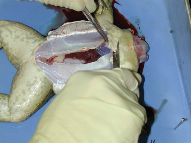
Figure 3:
Dissection of the frog showing the open
skin flaps, the removal of the sternum and, underneath, the exposed
heart inside the pericardial sack.
 |
- Obtain a pithed frog from the lab TA/Instructor and fix the frog on
its back using the big needles in the pan. Open the thorax of the frog
with a central incision and two flaps, which is also shown nicely
through a series of images in the web site
curry.edschool.virginia.edu/go/frog/Frog1/menu.html. Go to
the point of the Layer One section and focus on the heart. The point
here is not to perform a detailed dissection but to make you familiar
with the general anatomy and comfortable with the preparation of the
animal. Do not cut or remove any organs other than the skin
and some of the ribs covering the heart.
- To expose the heart, make sure to remove the lower and middle
sections of the rib cage as they will interfere with the transducer you
will use to measure contraction. The heart of the bullfrog is quite
large and red and should be slowly beating. Figure3
shows a the process of removing the ribs and sternum and the exposed
heart below. If the frog is still cold, the rate may be very slow so
run some Ringer's solution over the heart to help it warm up. Observe
the atria and single ventricle of the heart and note the sequence of
contraction of each.
- Once the heart is open, regular apply a few drops of Ringer's
solution to keep is moist.
- If you have a camera available, take photos of the thorax and mark
organs on them. If you do not have a camera, find images from a
classmate and label them for your lab report.
Figure 4:
Photo of the complete frog preparation
include the thread connecting the heart to the transducer.
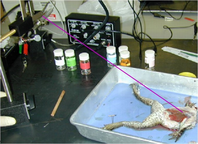 |
- Attaching transducer to the frog (See Figure 4):
- Very carefully, cut open and remove the pericardium from the
heart so you can see it fully exposed.
- Using the curved needle and suture provided, run the needle
through the lower part of the ventricle, about 5 mm from the apex
of the heart, and tie a loop with the suture thread. Then clip off
the needle and discard it carefully. Run the other end of the
suture through the hole in the transducer blade and tie a knot
there as well. Make sure there is at least 30 cm of suture
available between the heart and the force transducer.
- Place the transducer at the end of the pan, elevated about
about 20 cm above the table surface with the blade oriented
perpendicular to the table. The thread from the frog heart to the
transducer should be quit flat (horizontal) so that you apply
tension to the long axis of the heart. See
Figure 4 for reference.
- Apply a ground wire between the metal dissection tray and the
large metal plate on which you are working. This can reduce the
electrical noise levels substantially when we start to perform
electrocardiographic measurements.
- Now apply enough tension to the thread that you start to see a
signal on the oscilloscope that reflects the contraction of the
heart. Sensitivity of the 'scope should be in the range of
1-5 V/div. Adjust locations and tension so as to generate as clean
a signal as possible, ideally one that reveals the separate
components of atrial and ventricular contractions. Make sure the
tension of the thread is just enough to pull the thread taught and
lift the heart slightly, but not that it yanks the heart from the
animal. Check also that there is no obstruction from the side of
the pan or any other object. Place the pan and the stand well away
from the edge of the lab bench and always be careful not to
accidently touch the post or the thread so as not to change the
orientation or lose the reference signals, which will be important
later in the experiment.
Now, to visualize and acquire the electrical signals, carry out the
following steps. We will refer to the ``ECG'' or electrocardiogram to mean
the electrical signal acquired from the surface of the animal and the
``electrogram'' to be the signal acquired directly from the surface of the
heart.
- Arrange a second bioamplifier with the output going to the second
channel of the oscilloscope and the channel 2 of the A/D converter.
- Try the following settings on the bioamplifier:
- AC coupling
- A-B mode
- Low filter at lowest frequency setting
- High filter at low to moderate frequency
- Gain at or near maximum
First for the limb-lead ECG:
- Attach three wires from input of the bioamplifier to the needles
that attach the frog to the dissection pan. The green lead is the
reference and the red and black feed the signal to the bioamplifier.
Monitor the output of the bioamplifier on the oscilloscope and adjust
so as to get a clear signal.
- Try different arrangements of the wires and see which gives the
nicest and largest ECG signal, one that includes both atrial and
ventricular activity.
- Record the ECG together with the contraction signal and save on the
computer.
Figure 5:
Exposed heart with applied bipolar
electrodes. The electrodes should touch the exposed heart lightly.
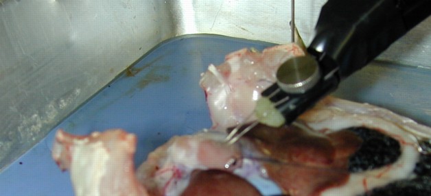 |
Now for the electrogram, the signal one can record directly from the heart
surface, as follows (see Figure 5):
- Take a bipolar electrode holder, attach it to a magnetic stand that
can lift up and down, and place the electrodes in contact with the
heart surface.
- Connect the wire from the electrode to a bioamplifier (use the
same one as previously for the ECG). Connect the reference lead to one
of the pins that hold down the feet of the frog.
Adjust the electrode location so as to get a clean signal of both
atrial and ventricular ``electrograms''.
- Record the electrogram together with the contraction signal on the
computer.
There are a set of interventions that you should carry out to see how the
heart responds to external stimuli, both mechanical and chemical.
Now try and replicate the effect of the Frank Starling mechanism with the
preparation by measuring contraction and progressively stretching the heart
to simulate the effect of increased venous return.
- Arrange the pan and transducer so that there is just enough tension
for the thread to clear the edge of the pan (adjust the height of the
transducer if necessary) and for you to get a contraction signal. Take
this as the baseline value and measure the applied force and the
amplitude of the contractions. Take a sample of data with the
computer.
- Move the pan a few millimeters further away from the transducer so
that it increases tension on the heart slightly. Then once again
measure applied force and contractile force amplitude and take a sample
of the signals on the computer.
- Repeat this process in 8-10 small steps until the heart
looks dangerously stretched, at each step recording applied force and
contractile response of the heart on the computer. Check with the TA
or instructor if in doubt about how far to stretch the heart.
- For the report, construct a plot of twitch contraction versus
pre-tension and explain which mechanism(s) explains the results. The
pre-tension is the base tension, which is visible in the force
transducer before (and after) the time-varying signal (twitch) from the
heartbeat. For the graph, you will need to make measurements of the
base level of the contraction signal as the independent (x axis)
variable. The dependent variable (y axis) you can then determine from
the peak contraction for each heartbeat by subtracting peak force
values from the pre-tension value. The resulting plot of contraction
versus pre-tension should look something like the Frank-Starling curves
from the text (or class).
- Note: make sure to apply the calibration curve to all the
data you acquire from the lab so that units are in grams or newtons.
Now dissect the heart from the animal and see if you can recognize at least
gross anatomical features like the chambers and major vessels.
- Remove the heart and attempt to open it up and see
structure.
- Remove lungs and attempt to inflate them, then slice them
open and observe structure.
After the lab you will have a lot of data from the tension and electrical
recordings from the frog and should now process, visualize, and analyze
these data for the report. MATLAB is probably the best tool for much of
this and is one tool that can do all of it.
Figure 6:
Example of the response to pre-tension.
The lower axes show two measurements of resting or pre-tension and
the resulting twitch tension during contraction. The inset graph
shows the resulting points in a twitch tension versus pretension
curve.
 |
Figure 6 illustrates one facet of the signal processing and
parameter extraction you should perform. The two time signals show
contraction under two different levels of pretension and the resulting
contraction tension. Note how the parameters from the time signals then
come together in a plot of twitch tension versus pretension--one form of
the Frank-Starling curve. You should construct a curve like this from your
own data.
Prepare just one lab report for this and the next lab together in which you
document your findings. For this section, include brief background and
methods sections and concentrate on showing the following:
- Labeled images of the thorax.
- Plots from the computer acquisition of contraction signal-please
use MATLAB to create these.
- Calibration curve for the transducer, which you should apply to all
the measured signals so that all plots are expressed in units of mass
(or force).
- Plot of contraction as a function of pre-tension (Frank-Starling
curve).
Wherever relevant, please attempt to describe and to interpret and discuss
your results. Did the results match your expectations? What are the
possible mechanisms for the response of the heart to contraction? Compare
atrial and ventricular contraction as you observed it in the frog heart.
The tips for homework assignments provided at
www.cvrti.utah.edu/~macleod/bioen/be6900/homework/homework-tips.html
also apply to lab reports.
Dissection and Contraction of Frog Heart
This document was generated using the
LaTeX2HTML translator Version 2002-2-1 (1.71)
Copyright © 1993, 1994, 1995, 1996,
Nikos Drakos,
Computer Based Learning Unit, University of Leeds.
Copyright © 1997, 1998, 1999,
Ross Moore,
Mathematics Department, Macquarie University, Sydney.
The command line arguments were:
latex2html -split 3 -no_white -link 3 -no_navigation -no_math -html_version 3.2,math -show_section_numbers -local_icons descrip
The translation was initiated by Rob Macleod on 2006-03-04
Rob Macleod
2006-03-04