The Macintosh Binary is an x64 build with Apple LLVM version 5.1
(clang-503.0.40)
Require Qt4.8 Framework to run.
Run this application from command line
User Interface:
The overall interface consists of two
views and one data operation panel. These visual components are
coordinated to provide a comprehensive view of the data by highlighting
its various aspects. They are interconnected such that selections and
changes made in one component will be reflected in others. The system is
designed to be modular and is easily extendable to include additional visual
components.
Embedding
View (a): This is the main
canvas of the interface where the results of DR, points embedded in 2D,
are visualized. It contains a rich set of user interactions for data
exploration. One could apply different colormaps to visualize points by
values of a particular dimension, clustering labels or point-wise
distortion measures. %In the case of visualizing local distortion, the
range of a colormap could be further adjusted by a percentage value to
accommodate new values that could be potentially out of range.
Parallel
Coordinate View (b): This
view displays the original data with each of its dimensions as a vertical
axis and each point as a line drawing through each of the axis. A
normalization of the range for each axis is optional to increase
readability of the data.
Data
Operation Panel (c): This
panel contains various data operations such as DR and clustering. The
panel is part of the interlinked system so that changes made to the
dataset are instantly reflected through other views. The panel consists of
three sub-panels: The meta-information panel gives a direct view of the
data, in terms of its dimensions and statistics, and includes the ability
to filter (hide) certain dimensions for analysis; The clustering panel
allows the user to select distance metrics, data standardization schemes
(see supplemental material) and hierarchical clustering methods (e.g.
classical single-, average-linkage), while also allowing loading of
existing clustering; and the DR panel enables the user to choose DR
techniques and specify their parameters in an online fashion.
File Format:
XML File Format
We use XML to store different kinds of meta information about the
data and the operations.
Import CSV file
Our system allows import of CSV data file with certain format
(defined as bellow).
The first line of the CSV file needs to be the label for each
dimension and separated by a comma.
Importing the file can be done by creating an empty file firstFile >
New and then import the CSV fileFile > Import CSV file.
Import external clustering results
Even though we provide several clustering method, we allow the user to
import any external clustering result.
The file needs to be a txt based label file, where each line
corresponding one point the dataset.
The label starting from zero, and there should not be label L exists
if there is no points belong to label L-1.
Import flat clustering can be done through File >Import
Clustering Result.
Data Operations:
Dimension Reduction
We provide a number of dimension reduction methods by interfacing with a
C++ template based dimension reduction library: Tapkee.
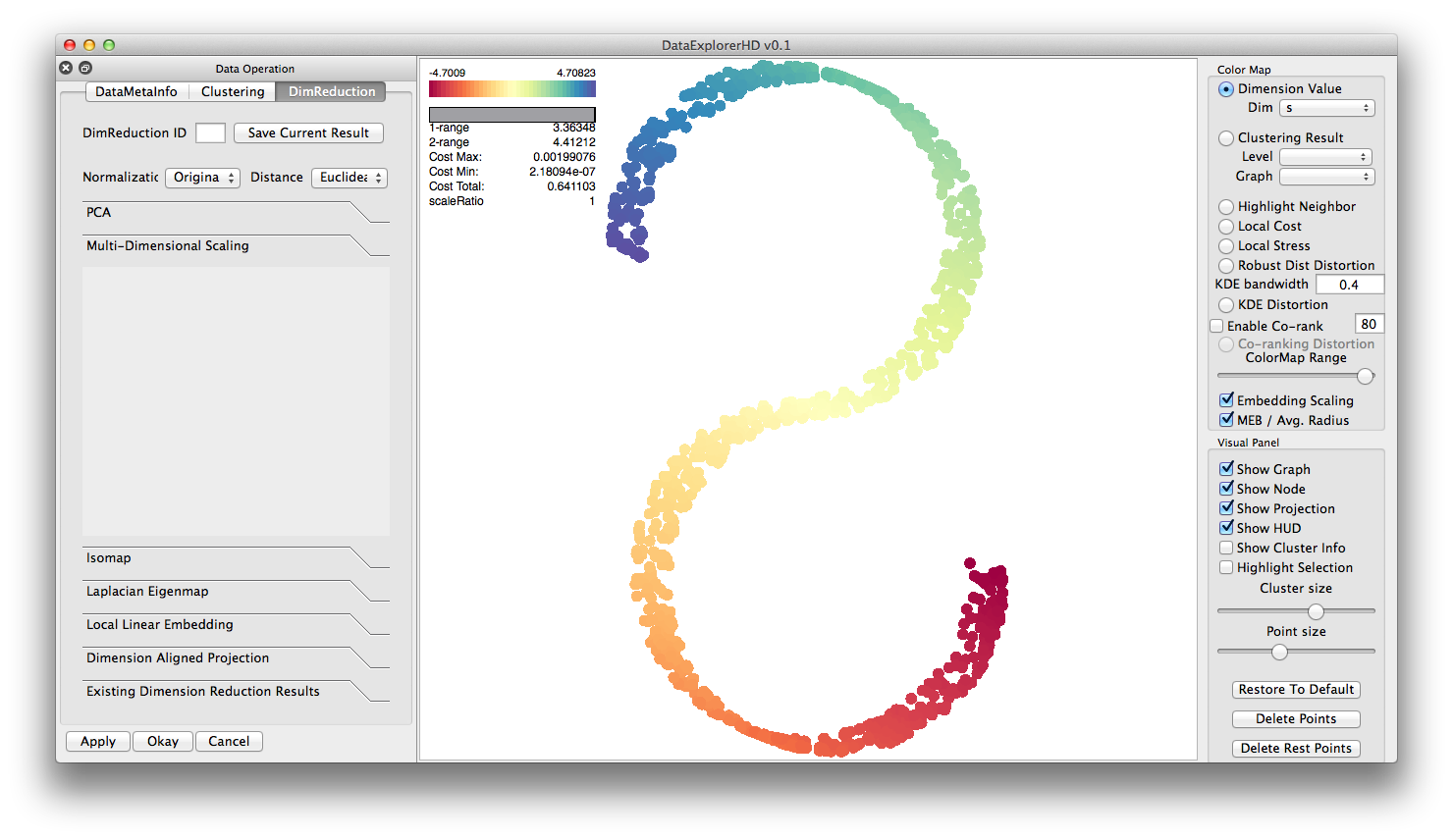
Here are some examples:
classical Multi-Dimensional Scaling ( S-curve dataset ):
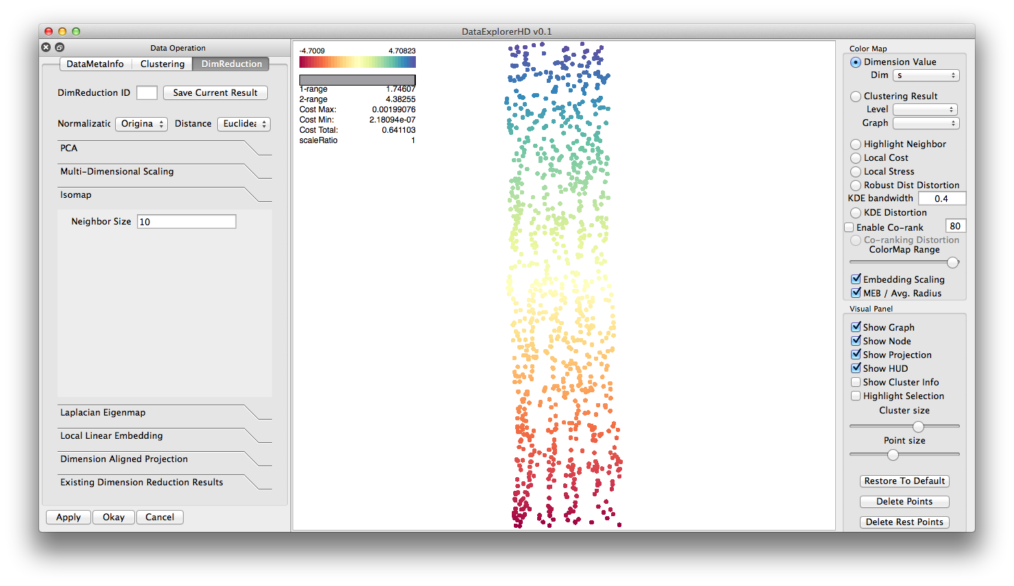
Isomap ( S-curve dataset ):
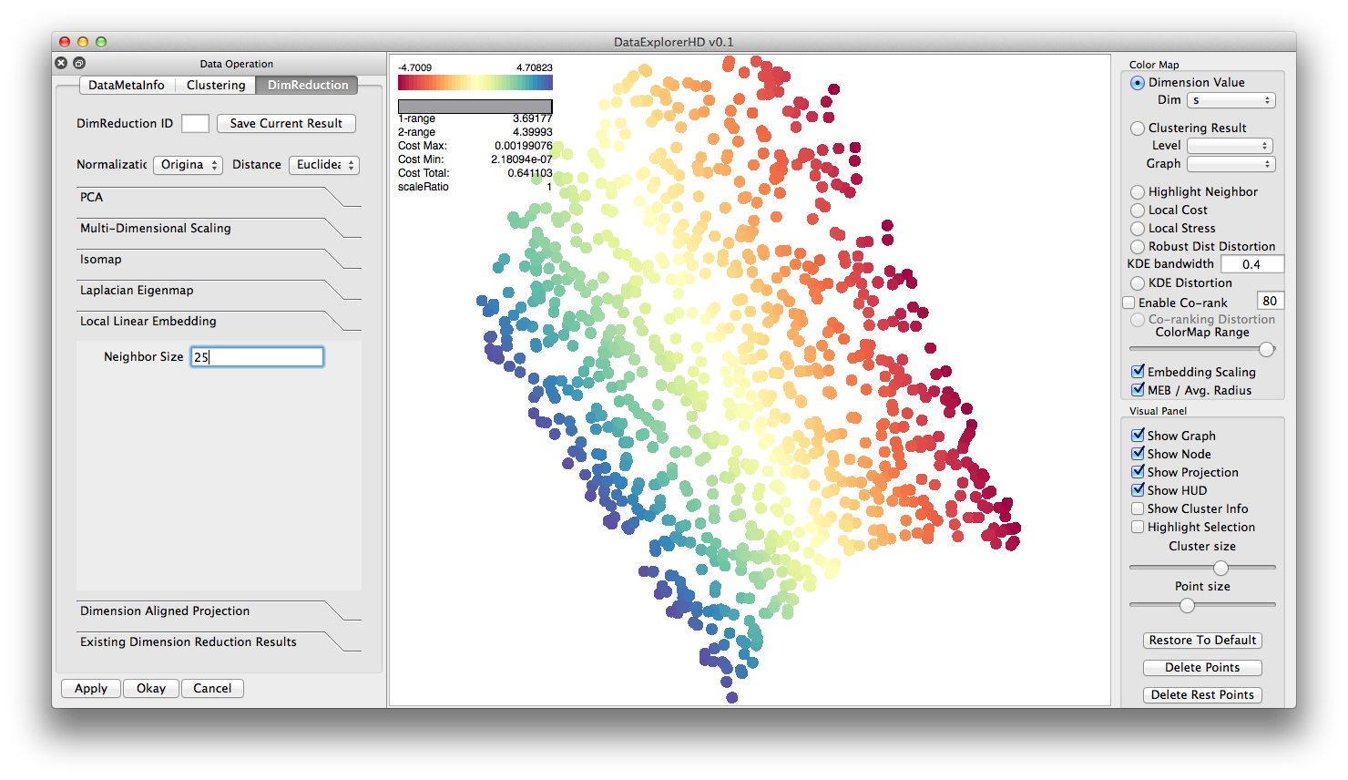
Local Linear Embedding ( S-curve dataset ):
Data Clustering
To aid the exploration and build skeletons for the manipulation in the
embedded space, we provide a number of different clustering methods.
Here are some examples:
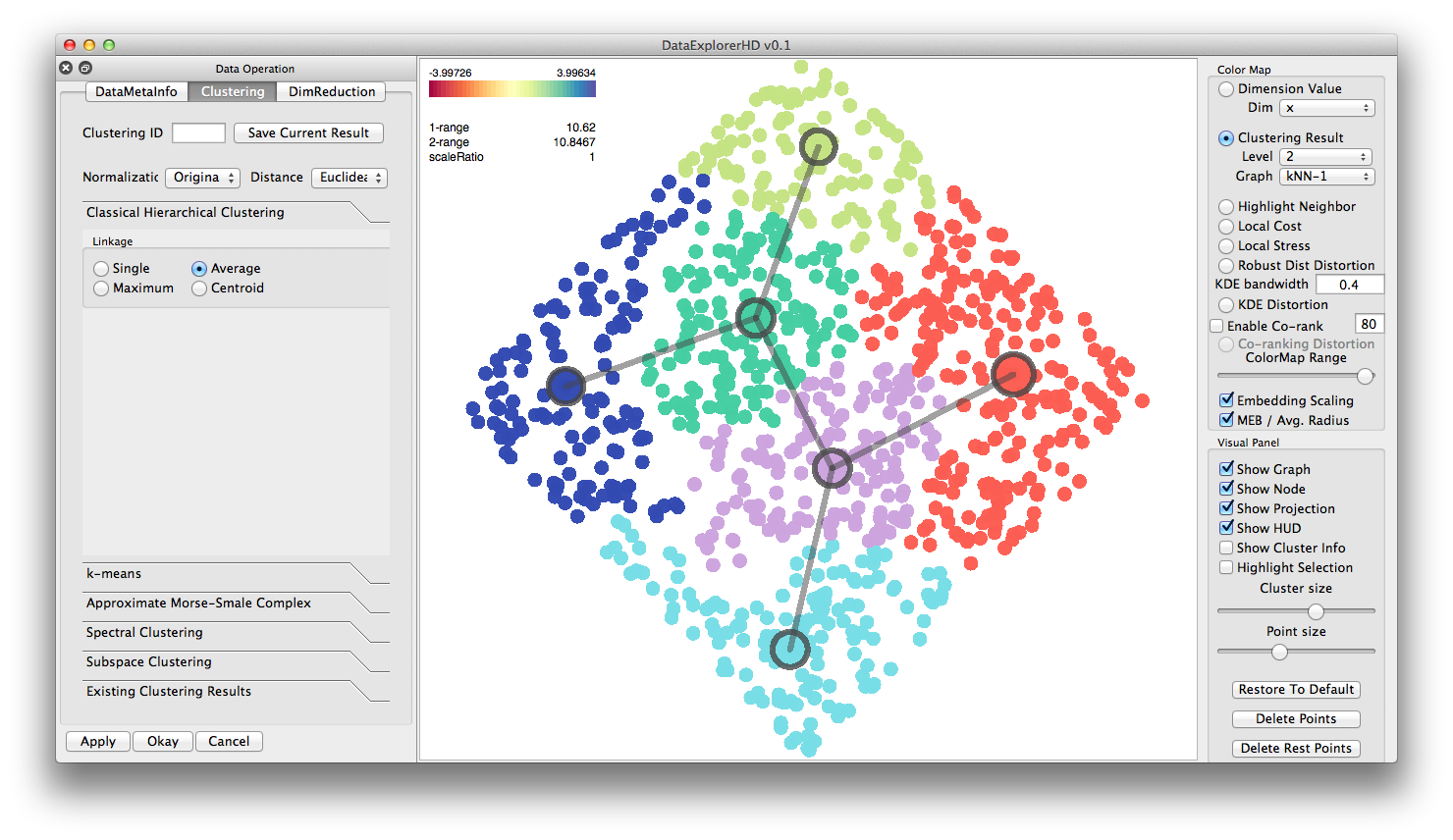
Classical Hierarchical Clustering ( Parabola dataset ):
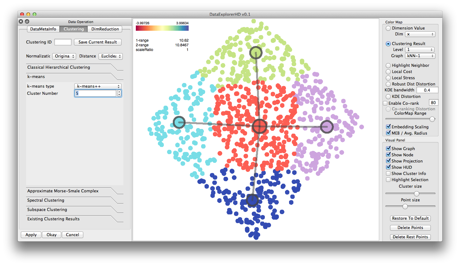
k-means++ Clustering ( Parabola dataset ):
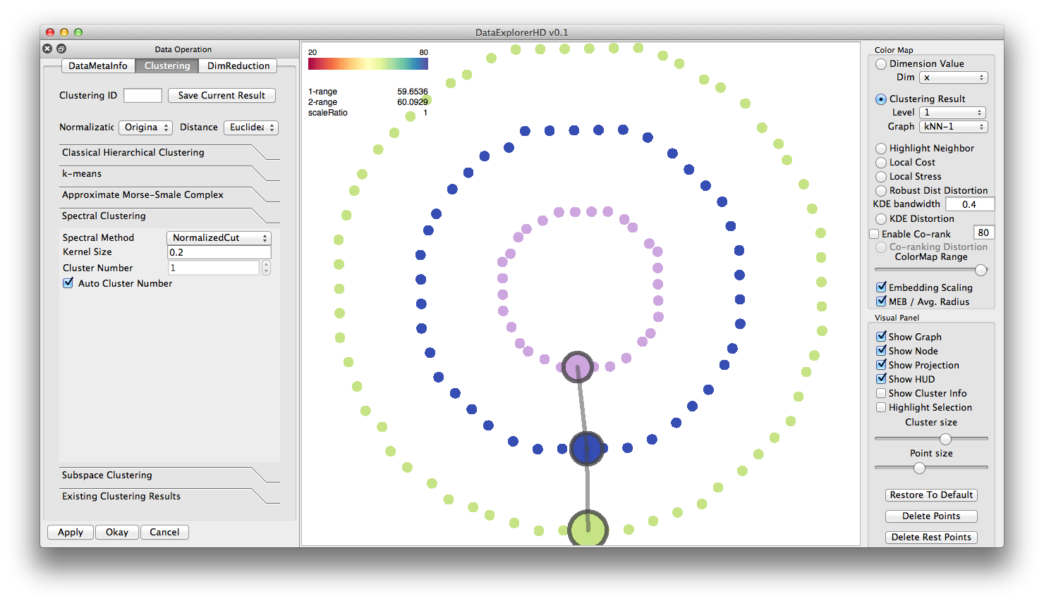
Spectral Clustering ( Circle dataset, with automatic clustering number
tuning):
Analysis Workflow:
Apply dimension reduction
Browse through different distortion measures
Apply clustering algorithm to obtain the structure skeleton
Utilize the structure skeleton for interactive exploration
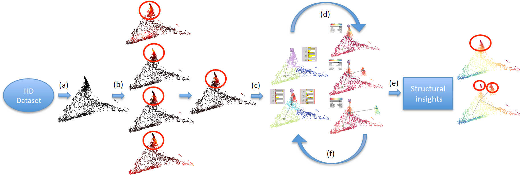
We illustrate a typical interactive exploration pipeline in above
figure.
(a) We
apply a certain DR technique to the high-dimensional dataset and
obtain its initial embedding, where global distortion measures such as
co-ranking could be employed to select a suitable DR and its optimal
parameter setting.
(b) We visualize point-wise
distortions on the embedding. Regions with high distortions across
multiple measures (for example) are identified as regions of interest
for further investigation.
(c) We apply hierarchical
clustering of the data.
(d) We use point-wise
distortions to guide our clustering selection, where the appropriate
level of clustering is chosen based on its agreement with the region
of interest.
(e) We allow users to move
and/or delete a subset of data that belongs to a targeted
cluster in the visual space,
where on-the-fly updates of point-wise distortion measures reflect
structural relations between different parts of the data.
A decrease/increase in distortion measure of the targeted cluster
typically indicates structural independencies/dependencies among the
target and its neighboring clusters.
(f) In addition, with detailed
parameter analysis across each cluster, we obtain further insights
regarding differentiating factors among different regions of the data.
Finally, we obtain a collection of structural insights.
The video from our paper explain the
analysis workflow in details: