Point Sample Rendering

The MLS surface
Overview
Projection

Applications

Results

Download
Vis'01 pss.pdf
TVCG crpss.pdf

progressive pss ppss.pdf

Marc Alexa
Johannes Behr
Daniel Cohen-Or
Shachar Fleishman
David Levin
Caludio T. Silva

Abstract

We advocate the use of point sets to represent shapes. We provide a definition of a smooth manifold surface from a set of points close to the original surface. The definition is based on local maps from differential geometry, which are approximated by the method of moving least squares (MLS). We present tools to increase or decrease the density of the points, thus, allowing an adjustment of the spacing among the points to control the fidelity of the representation.

To display the point set surface, we introduce a novel point rendering technique. The idea is to evaluate the local maps according to the image resolution. This results in high quality shading effects and smooth silhouettes at interactive frame rates.

The MLS surface definition

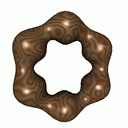
A given point set implicitly defines the MLS surface. The main idea of the MLS surface definition is a projection procedure, which projects any point in the neighborhood of the surface onto the surface. A projection procedure F is such that F(x)=F(F(x)). Therefore, we define the MLS surface that is defined by an input set of points as the set of points that project onto themselves.

Let points P={p_i} be sampled from a surface S (possibly with measurement noise). The goal is to project a point r near S onto S_p, the MLS surface defined by P. The projection procedure is motivated by differential geometry, namely that a surface can be locally approximated by a function.

To project r onto S_p, a three step procedure is performed:

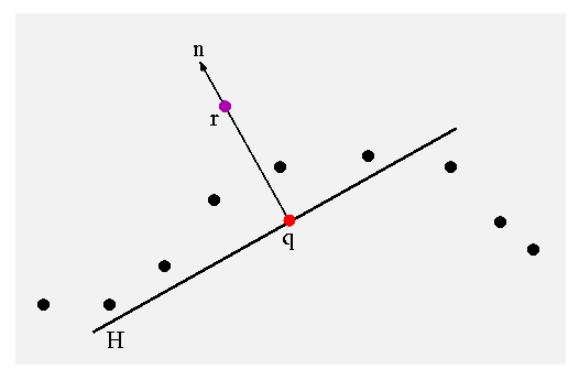
1. A reference domain H is computed by minimizing eq. 1.
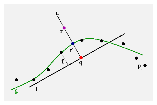
2. The reference domain defines a function in the neighborhood of r (the f_i's in Figure 1b). A local polynomial g is fitted through the points in the neighborhood of r.
3. The projection r' of r is computed using eq. 3.

Where n is the normal to the plane, D is the distance of q from r i.e. D=||r-q|| and q is a smooth, radial, monotone decreasing function, which is positive on the whole space. The local reference domain is then given by an orthonormal coordinate system on H so that q is the origin of this system.

The reference domain for r is used to fit a local bivariate polynomial for r through the points in the neighborhood of r (See Figure 1). To compute the polinomial g, a least squares approximation is used to minimize equation 2.

N å i=1  ( g(xi,yi) - fi ) 2 q( || pi - q || )

(2)

Where <x_i,y_i,f_i> are the coordinates of p_i in the coordinate space of the reference domain H and q is the same weight function as above.

 

r'=MLS(r) = r+(t+g(0,0))n.

(3)

(a)	(b)
Figure 1: First, a local reference domain H for the purple point r is generated by searching for the point q that minimizes eq. 1. Then a local polynomial g is fitted to the height fi of points pi over H.

The key observation in the MLS projection procedure is the computation of the reference domain. Observe that all of the points (in the neighborhood of r) along the normal n share the same reference domain H.  

The importance of the projection operator

• Point-based modeling: the MLS surface is a point-based surface definition that is continuous and smooth.
  • Noise removal
  • Object smoothing
  • Object resampling (reparameterization)
  • Upsample and Downsample for modeling and rendering
  • High quality normal and curvature estimation
  • Accurate ray-tracing of point-based objects
• The local reference domain defined by the MLS projection procedure gives rise to many algorithms typically applied to planar objects.
  • Texture growing
• The projection operator allows us to simplify known algorithms:
  • Scattered data meshing
  • Object sampling using particles systems.

(a) (b) (c)

Regular resampling of the Buddha model (courtesy of Stanford 3D scanning repository), (a) is the unevenly sampled input model . (b) is the resampled model at regular intervals. (c) is a rendering of the resampled model.

Point-based rendering of the angel model

Venus

High quality zoom on Venus
Adding points by projection of new points in the neighborhood of the object