

Advanced Image Processing
Project1: Scale-Space Selection, Spring 2010, CS7960
Xiang Hao
1. Blob segmentation by scale selection
1.1 Create scale space
In order to create a scale space, as I know there are at least two equivalent methods. Gaussian diffusion or solve a heat equation.
For the latter method, I just learnt from the recent AIP class and I haven't implemented it before, but fortunately I will have a chance to implement in project2.
For the former method, I implemented it as the Dr. Gerig suggested:
1) Create a array of t. For example, t=1:0.1:3.
2) Compute the sigma as exp(t)
3) Create a bunch of Gaussian filter with different sigma.
4) Convolve the image with the different Gaussian filters, and we will get the scale space.
1.2 Laplacian filtering
In my opinion, this is the major idea of this detection.
At first, I am wondering why the laplacian filter can detect the blob, why it will has a maximum response at certain scale, and why the response will first increase and then decrease.
These questions confused me a lot, but after several discussions with classmates, I think I've understood part of it.
The straightforward explanation is that: suppose a blob has the fixed size. If we use different laplacian filter with different width, we will get different response. The maximum response will happen when the width of the laplacian has certain value. This value is related with the size of the blob.
Yes, the above explanation is easy to understand, but it still does not answer my question: why does the laplacian filter have a maximum response at certain scale since we are using a single laplacian filter?
After a further thinking, I realize that the size of the blob and the width of the laplacian are relativistic. In this project, thought the width of the laplacian filter is fixed, the size of the blob is decreasing through scale space. This is why the laplacian can dectect the blocs by scale selection and I am wondering if we can use different laplacian filters to detect the blobs rather than use the scale space. I guess the answer is yes.
1.3 Maximum detection strategy
As I said in the last part, the laplacian filtering is the major idea of this detection, but this part is the most tricky part.
How to find the maximum?
First, we need to find the local maximum at each scale space. This is the first step. When finding the local maximum, we will find a lot of local maximums, which are not quite right. For examples, we will find a lot of local maximums forming a circle. We want to eliminate these local maximum since we only want to find the real peak. I implemented it by comparing the local maximum with its neighbor(we can change the size of its neighbor). For every pixel of the image, if the intensities of it neighbor is decreasing from the center, I treat this pixel as a local maximum.
The next step is to find the maximum response in the scale space.
I did in this way,:
1) At a scale, we find the first bunch of local maximum and add them to the candidate points list, see list L. Be careful, we may not find a local maximum in the first scale.
2) At the next scale, we will find another new bunch of local maximum. Then I compare the position of new local maximum with the candidate points which are already in the list L. If the new local maximum is far from the candidate points, I will add the new local maximum to the list L. On the other hand, if it is close to some of the candidate points, I will compare their intensity. The one who has larger intensity will be add to the list and the one who has lower intensity will be delete from the list L if it is in the list L. Keep doing this until the last scale space.
By the above two step, I can find the maximum response very well.
2.Results
1)Blurred image
|
|
|
|
|
|
|
|
|
2)Laplacian filtering
The images after laplacian fitering have some negative value. When save the image, the matlab discard the negative value, so the following images are not accurate.
|
|
|
|
|
|
|
|
|
List of the circle centers:
x , y, scale level , intensity
45.0000 44.0000 15.0000 186.1988
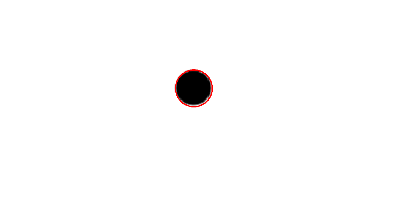
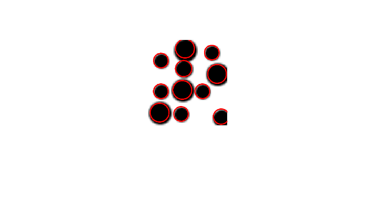
Final result
|
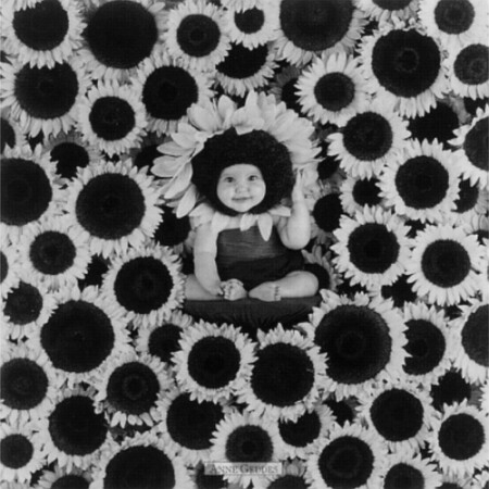
Original Image |
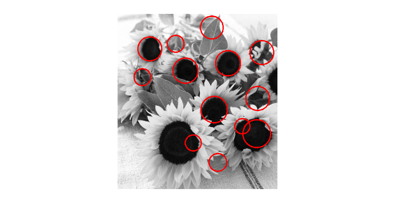
Blob segmentation results |
|
|
|
|
|
|
|
|
|
|
|
|
Parameters to get the above results:
|
Image1 |
Image2 |
Image3 |
Image4 |
|
t_array=1:0.1:3; coef_gau_filter=1.8; coef_peak_mask=9;
|
t_array=1:0.05:3; coef_gau_filter=1.8; coef_peak_mask=9; |
t_array=1:0.1:3; coef_gau_filter=2.0 coef_peak_mask=49; |
t_array=1:0.1:3; coef_gau_filter=2.5; coef_peak_mask=29; |
3. Discussion
Generally, the results is quite well as we can see from the above picture.
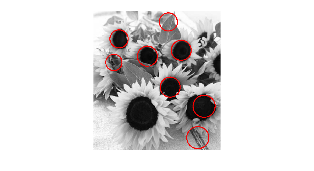
Especially for the last image, it can detect every circle! This result is very exciting.
For the fist two pictures, the algorithm can detect all of the circles, the radius of the circles are good, but some of them are not that accurate.
For the third picture, the result is not as good as the first two synthetic picture. There are some wrong circles and it missed some circles.
For the last picture, the result is pretty good. It can detect every circle. There are some half circles in the the figure, but my program did not find them and it also has some wrong detections.
These wrong circles are probably caused by the irregular shape of the circles and some noises.
4. Comments
There are some issues when we implement this algorithm:
1) The size of the Gaussian filter is important.
For example, if the size is very small, the image will not be blurred enough. In this cae, when we use a laplacian filter, we will get a bigger value. Since we need to normalize the image by multiplying sigma^2. So we will get a very high value in the high scale space. This means the response will increase all the time. It will not first increase and then decrease if the image is not blurred enough.
2) The interval between two scales.
The smaller the interval is, the accurate our result is. So if we want to improve our results, we may decrease the interval, but this will cost more time. It is a trade off between accuracy and time cost.
For example: the right result is better than the left one.
|
t=1:0.1:3 |
t=1:0.05:3 |
|
|
|
3)The size of the neighbor.
We can use small neighbor, but if the neighbor, we may find a lot of small circles. So the neighbor should not be small. In a complicated image, if we do not want to find many wrong small circles, the neighbor should be large enough, but this is still a trade off between accuracy and time cost.
For example: the right result is better than the left one.
|
neighbor=39 |
neighbor=49 |
|
|
|
Potential improvements:
1)Use head equation rather than using Gaussian filter.
2)We may use Subirana Vilanova's method to improve the accuracy of the circle center.
Matlab codes are here.