What?
Physical Phenomena
Mathematical Model
Simulation
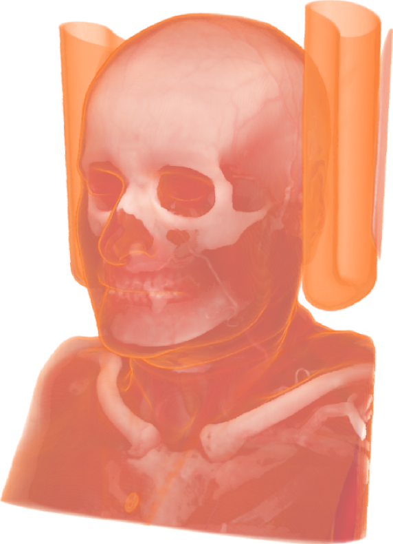
Visualization
Tiago Etiene | University of Utah
Mike Kirby | University of Utah
Cláudio Silva | NYU-Poly
Example: \( I(x,y)=\int_0^D C(\lambda)\tau(\lambda) \times \exp\left(-\int_0^\lambda\tau(\lambda') \mathrm{d}\lambda'\right)\mathrm{d}\lambda \)
\( \qquad \qquad \quad~ = \sum_i^n C_i \tau_i d \prod_j^{i-1} (1 - \tau_i d) + \) \( O(d) \)
Generally: \( I(x,y)= \tilde{I}(x,y) + \) \( O(d^k) \)
How the order of accuracy will change when different approximation schemes are used?
We will not talk about how the discretization errors affect the quality of the rendered image (the evaluation question)
Ground truth: \( C, \tau, s, \) and the analytical solution \( I \) of the VRI are known
Approximation: given \( C, \tau, \) and \( s \), \( \tilde{I} \) is numerically computed
Approximation errors are computed as: \( |\tilde{I}-I| \)
\( I(x,y) = \int_0^D \alpha(s) \exp \left( -\int_0^s \epsilon(s') \mathrm{d}s' \right) \mathrm{d}s \)
Assuming that \( \alpha(s) \) and \( \epsilon(s) \) are approximated by polynomials:
\( I(x,y) = \int_0^D p(s) \exp \left( q(s) \right) \mathrm{d}s \)
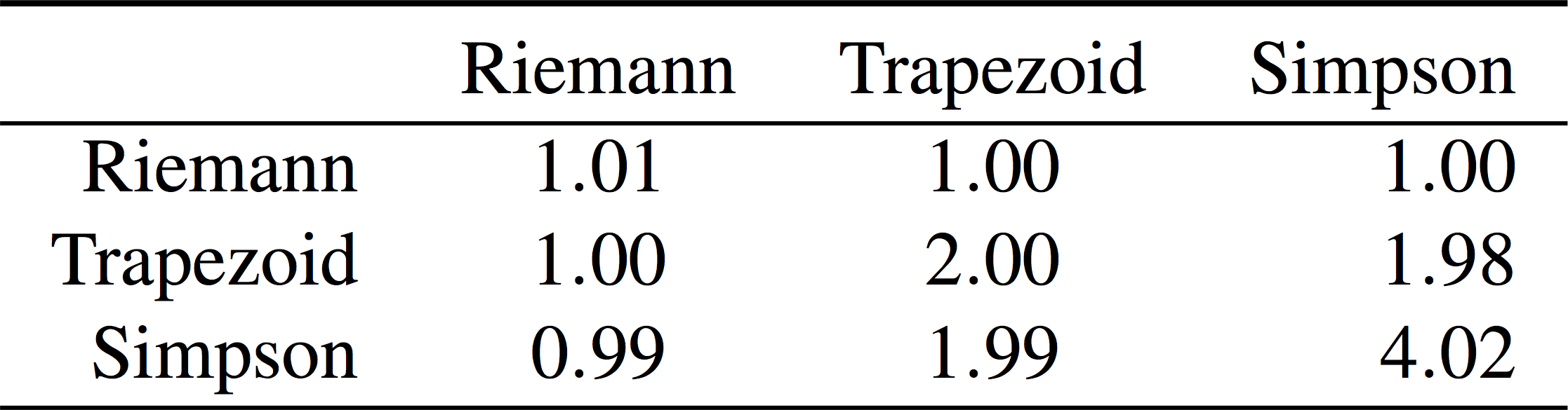
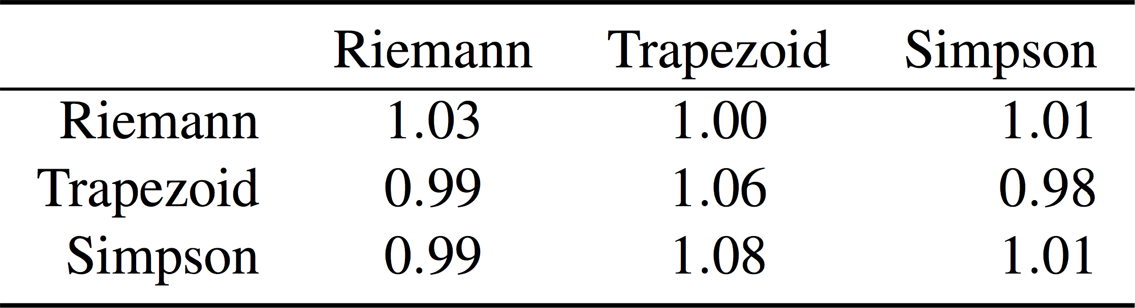
The order of accuracy will depend on \( p, q, \) and the approximation of the outer integral: Trapezoid, Simpson, or Power Series.
Convergence rate is given by \( \min(p, q, r-1) \), where:
\( f_{\text{inner}} = \tilde{f}_{\text{inner}} + O(d^p) \)
\( f_{\text{outer}} = \tilde{f}_{\text{outer}} + O(d^q) \)
\( e^{-f_{inner}} = \tilde{e}^{-f_{inner}} + O(d^r) \)