Introduction
The objective of this first project is to develop and implement some image processing functions based on the histogram of an Image.
In a first part we will present briefly some theoretical aspects associated with histograms and the processing associated. Then we will present the different functions and processing we developed for this project.
We will try to explain and present all the results and the step we've been through in this project.
Note: The following MATLAB functions are associated to this work:
Note: The code evolved a lot while I was writing this report, so some images produced may not be the exact same as the one I've used in this report. The structure of this report is following the subject but sometimes I have considered several questions at the same time.
Note: Some images were provided for this project, for the MRI image I used, I don't have any right on it, it comes from a MRI database. I made all the other drawing or images so there is no Copyright infringement in this work.
Theoretical definitions
I: Image
A digital image is a discrete space composed of small surface elements called pixel. Each one of this elements contains a value or a set of value coding the intensity level at each position. A digital image can be acquired with a great number of different devices such as a camera, an MRI machine or any kind of device with a sensor able to capture light intensity.
Because of its discrete nature, the theory used to process digital image will rely on discrete domain, even if the analogy with the continuous domain is possible.
A: Gray scale digital image
A gray scale image is a digital image in which each pixel only contains one scalar value which is its intensity. The number of possible levels (intensity values) depends on the numerical type encoding the image.
For example, an image encoded with n=8 bits will only have L=28=256 possible intensity values going from 0 representing black to L-1=255 representing white.
B: Color image
A color image is a digital array of pixel containing a color information. Each image can be decomposed into three different layers according to the three color channels encoded: Red, Green and Blue.
For instance, a 8 eight bits color images encode the Red and Green channel with three bits and the blue with two. Which could encode 256 different colors.
II: Histogram
The histogram of a digital image is a distribution of its discrete intensity levels in the range [0,L-1]. The distribution is a discrete function h associating to each intensity level: rk the number of pixel with this intensity: nk.
III: Transformation of Histogram
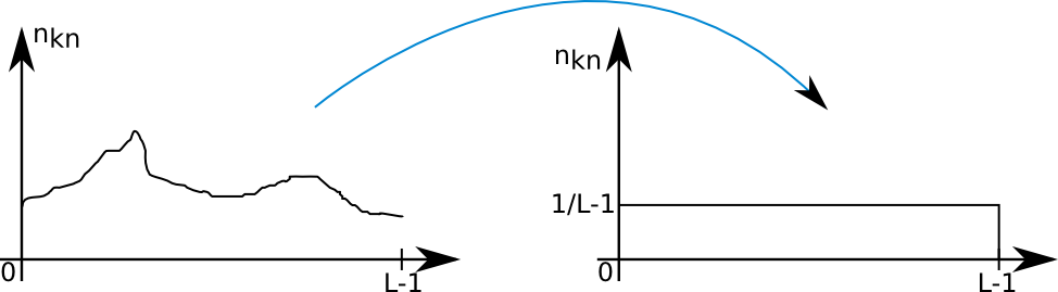
A: Normalization of a Histogram
Normalize an histogram is a technique consisting into transforming the discrete distribution of intensities into a discrete distribution of probabilities. To do so, we need to divide each value of the histogram by the number of pixel. Because a digital image is a discrete set of values that could be seen as a matrix and it's equivalent to divide each nk by the dimension of the array which is the product of the width by the length of the image.
\[{n}_{kn}=\frac{{n}_{k}}{length \times width} = p_{r}(r_k) \]
Which could be written in terms of mathematical transformation:
\[\begin{cases}[0,L-1] \rightarrow \mathbb{N} \\ x \rightarrow Card(x) \end{cases} \quad \text{becomes} \quad \begin{cases} \quad [0,L-1] \rightarrow [0,1] \\ \quad\ x \rightarrow pdf(x)=\frac{Card(x)}{\sum_{i=0}^{L-1}Card(x_i)} \end{cases} \]
Where Card means the cardinality of the set so in our case the number of pixel.
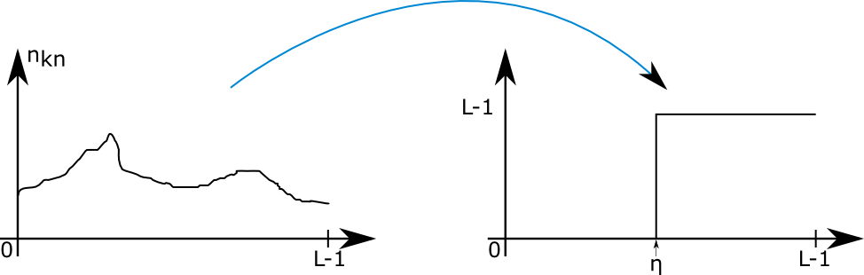
B: Equalization of a Histogram
Histogram equalization is a method to process images in order to adjust the contrast of an image by modifying the intensity distribution of the histogram. The objective of this technique is to give a linear trend to the cumulative probability function associated to the image.
The processing of histogram equalization relies on the use of the cumulative probability function (cdf). The cdf is a cumulative sum of all the probabilities lying in its domain and defined by:
\[ cdf(x) = \sum_{k=-\infty}^{x} P(k) \]
The idea of this processing is to give to the resulting image a linear cumulative distribution function. Indeed, a linear cdf is associated to the uniform histogram that we want the resulting image to have.
So we are going to implement the following formula to get the new pdf:
\[ S_k=(L-1)cdf(x) \]
C: Segmentation with an histogram
Segmentation is an operation consisting in partitioning an image into sets of elements. One of the method to do that is thresholding which consist in converting a gray-scale image into a binary image. The most important step here is to chose the best value for the threshold to get the best segmentation. Several methods exists to determine it.
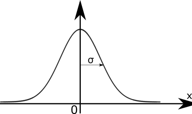
IV: Gaussian or Normal distribution
The Gaussian probability distribution function is a kind of pdf defined by:
\[ \begin{cases} \mathbb{R} \rightarrow [0,1] \\ G_1(x) = \frac{1}{\sqrt{2\pi}\sigma}e^{\frac{-(x-\bar{m})^2}{2\sigma^2}} \end{cases} \]
with \[ \bar{m} \text{ being the mean and } \sigma \text{ being the standard deviation} \]
Programing
For this project, all the programming to process images and create the results associated to each experiment is made with MATLAB. MATLAB is a numerical computing environment developed by MathWorks. MATLAB allows matrix manipulations, plotting of functions and data, implementation of algorithms and a lot of many other things.
More information :
http://www.mathworks.com/products/matlab/index.html
So all the code I'm going to present here is using matlab programing language syntax. But all algorithm will work with any other languages. A more detailed presentation of the code is available in the Implementation section.
Build a Histogram
An histogram being a distribution of the number of pixel according to their intensities, we have in this part to analyze the image to determine this distribution. Then we will perform some other operations to allow the user to enter the number of desired bins for the histogram and the range of values that should cover the histogram.
We developed a function that is taking as input a 2 dimension array (a digital image) containing for each pixel an associated intensity value. The type used to store these values can either be integers or floats. The function is converting this 2 dimension array into a single dimension array containing the frequency of each intensity level.
To get this histogram here is the algorithm we implemented:
For each pixel of the image
    value = Intensity(pixel)
    histogram(value)++
end
In the previous result, we are just displaying the absolute frequency which is the number of pixel. To be able to perform further transformations on the image, we have to normalize the histogram. The normalization will give to our distribution the properties of a probability density function. To get this result, we used the formula given in the theoretical part.
The objective in this part is also to be able to modify the different parameters of the histogram. Indeed, we want to be able to specify the number of bins and also its range. So we need to determine the size of each new bin and then perform a test on the value of the histogram to find in which bins it lies. To compute the size of the new bin, we use the following formula:
\[binsize = \left [ \frac{\max - \min }{n} \right ] \]
Note that in this case we consider a rounding for computing the size. The brace uses Kenneth E. Iverson notation of the rounding function.
The algorithm to parametrize the binning of the histogram is:
define bin width
For each value read from the image
    value belong to [min,max] interval ?
      if yes find in which bin and increment bin
      else return
      end
end
So the final function we produced is taking an image as input and providing an histogram with a specified number of bins and range. Examples are provided in the following section.
Experimentation
In this section, we are going to show different histograms associated to different images and try to explain and interpret them in regard to the image we gave as input.
I: Grey scale digital image
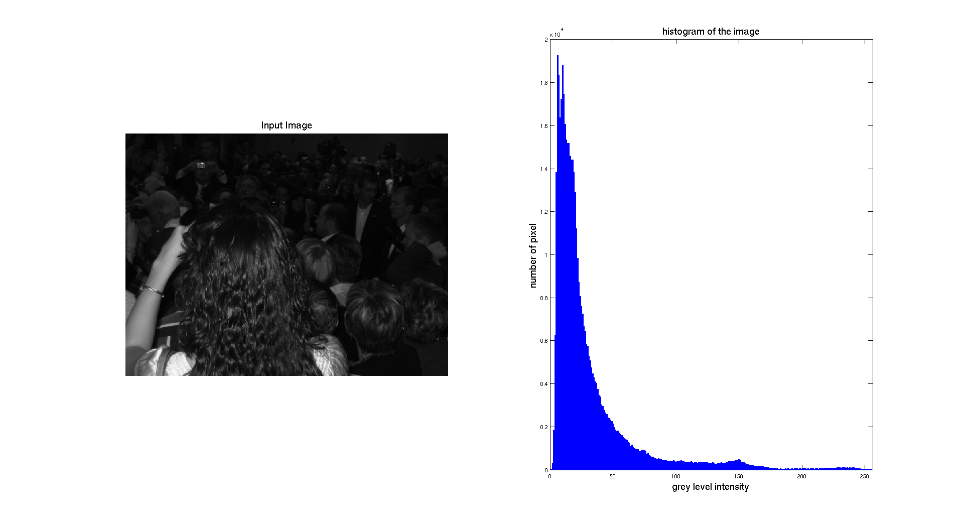
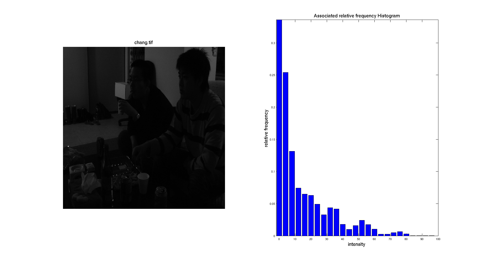
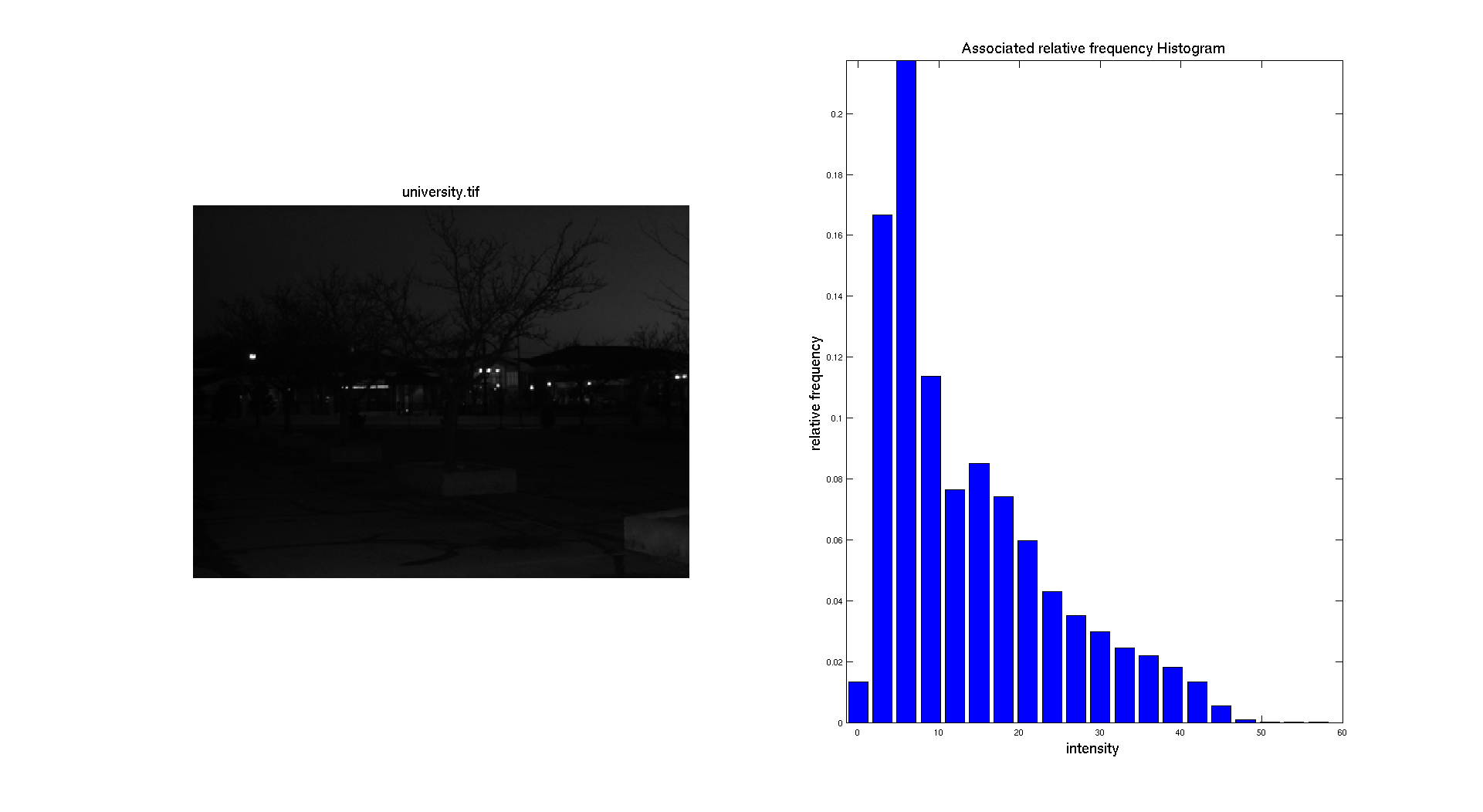
So let's start with an experimentation on the pictures given for this project
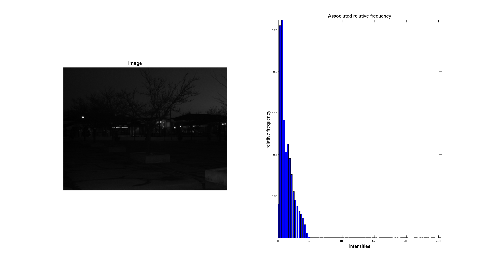
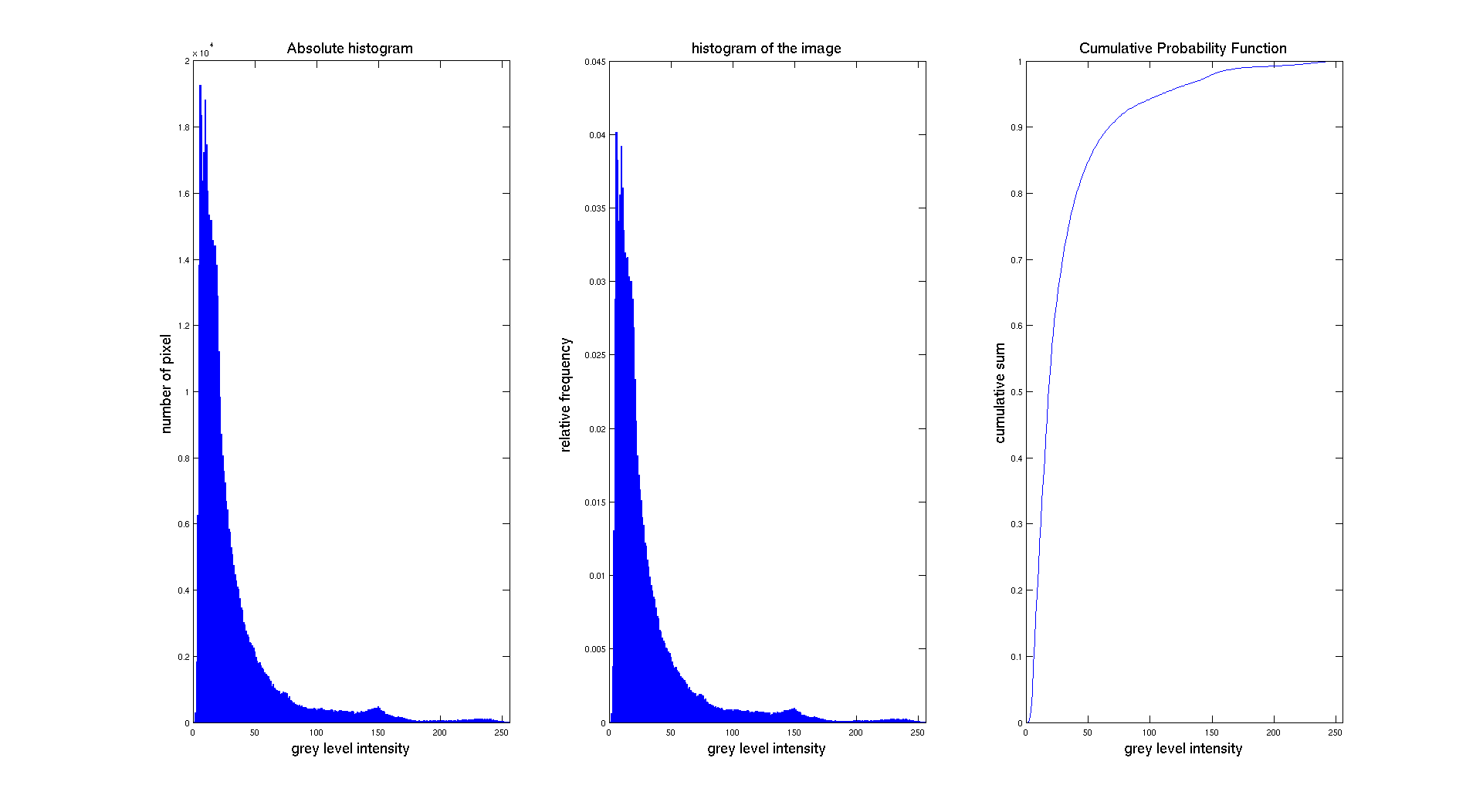
On the previous figure, we can see that the input picture is really dark. We can see this aspect while looking at the associated normalized histogram where we can see that the histogram is located on the left side which correspond to the darkest gray levels.
If we consider a different image, like the CT scan the result is pretty different:
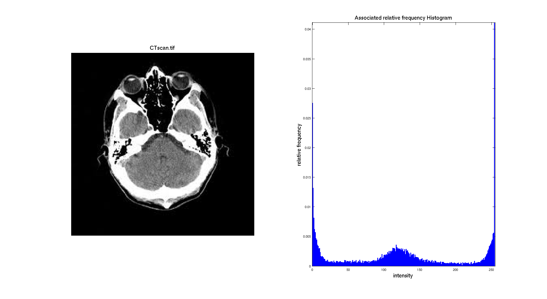
Indeed, on that image the skull of the head is clearly appearing white and there is also a huge number of pixel with an intermediate gray level. The background is black and is representing a big part of the image. So it makes sense to have three different "regions" on the histogram: a big peak for black made with the background and some part of the head, a gray "region" composed of the pixel from the brain and a white region with the pixel of the skull.
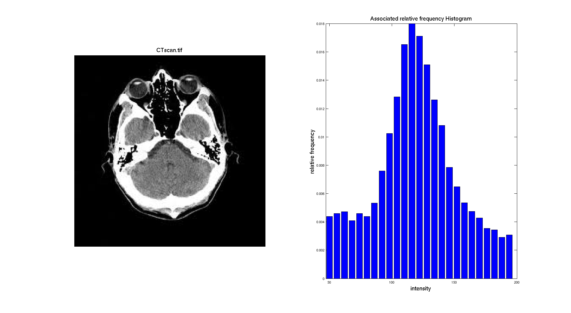
Let's apply here a restriction on the range of the histogram we are displaying so it only focuses on the regions corresponding to the middle range of the histogram i.e the brain. So we are considering only the range of values between 50 and 200.
We can also generate the histogram of the other images. With an intensity range going from 0 to 100 for chang.
II: Color image
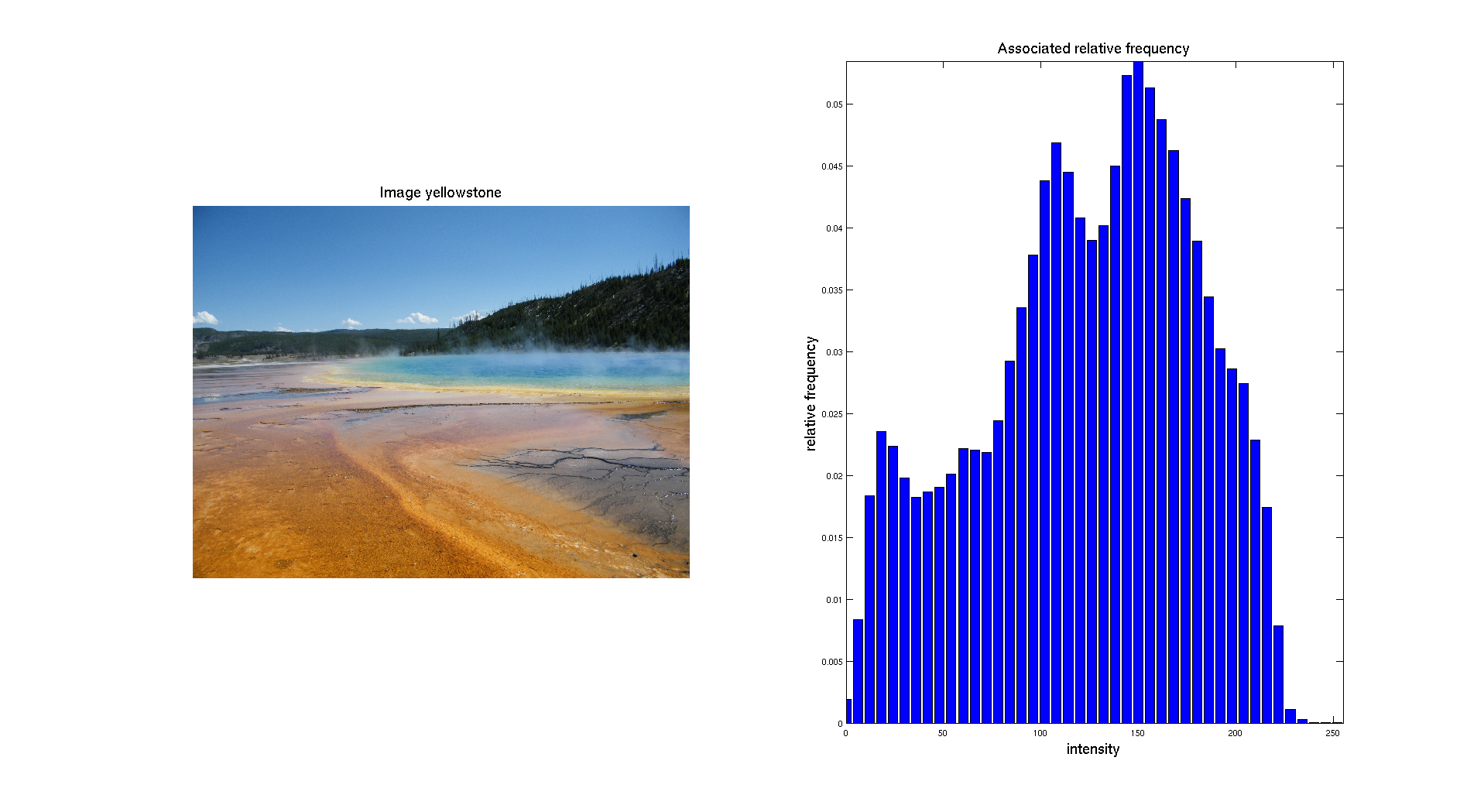
We can also give as input a digital color image. Then the first thing to do is to separate the three different color channels: Red, Green and Blue. Let's take as input a picture I took of Grand Prismatic Lake in Yellowstone National Park.
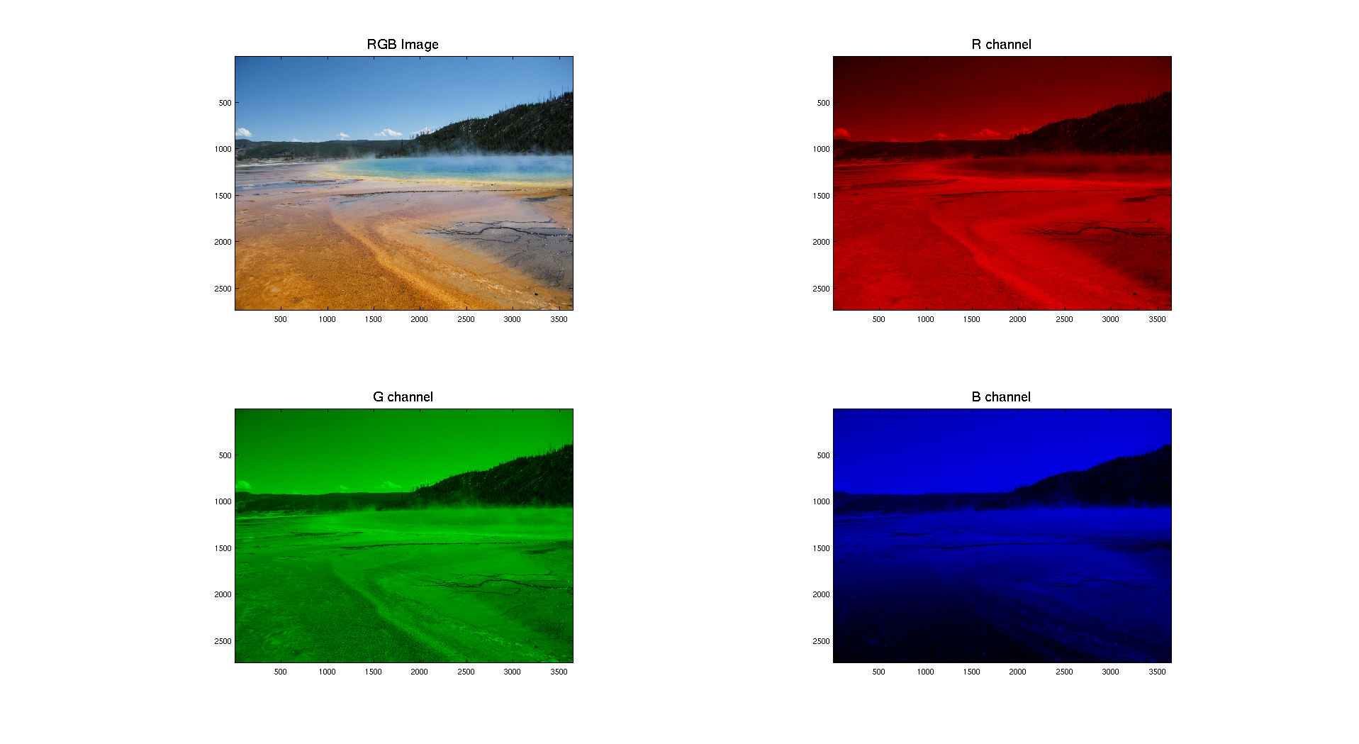
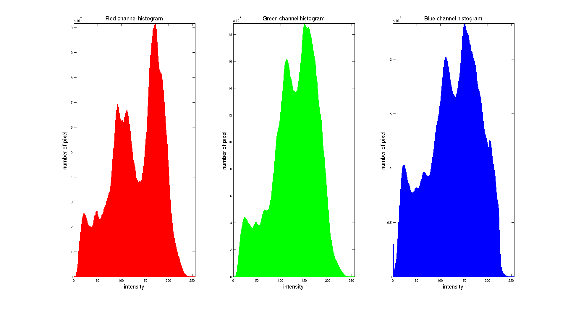
Here we can clearly see that the distribution of the intensity on each channel is clearly different. The color image is obtained while combining the three layers. We obtain the following result:
Histogram Equalization
In this part we are only going to consider Gray scale images. As we have seen before, some images are really dark and have their histogram concentrated on the lower values of the intensity. So the objective of this part is to enhance the contrast of the image by equalizing the histogram.
To perform this operation, we are going to implement the formula presented in the section IIIB of theoretical part at the beginning of this report. To do so, we will need to perform as a first step the computation of the histogram of our input image. To do so, we can call the function histogram we have already implemented in the previous part. A detailed explanation of the code is available in the Implementation part.
I: Results
Here are some results and comments for the images given.
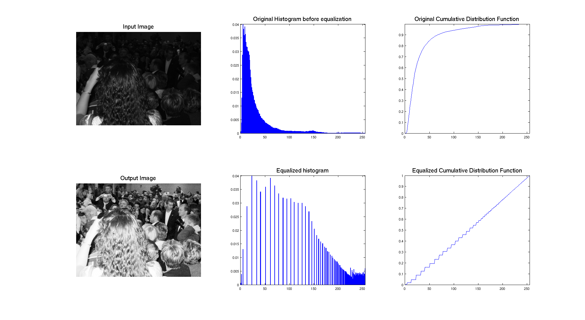
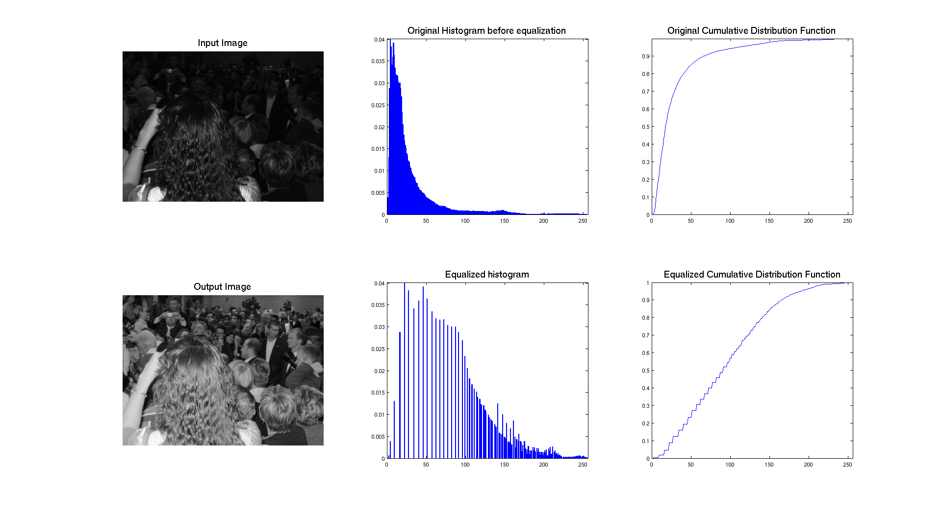
As we can see on the previous figure, if we compare the two images we can see that the contrast of the image has clearly been enhanced by performing equalization. The success of the procedure is proven by the histogram associated to each image, showing that it's range has been stretched to occupy the whole spectrum of levels. We also have an expected result for the cumulative distribution function because we have an almost linear cdf.
In terms of qualitative judgment on the image, we can clearly see that the contrast is better because we are now able to see what was at the background and that the picture is really showing a crowd, which was not that obvious before.
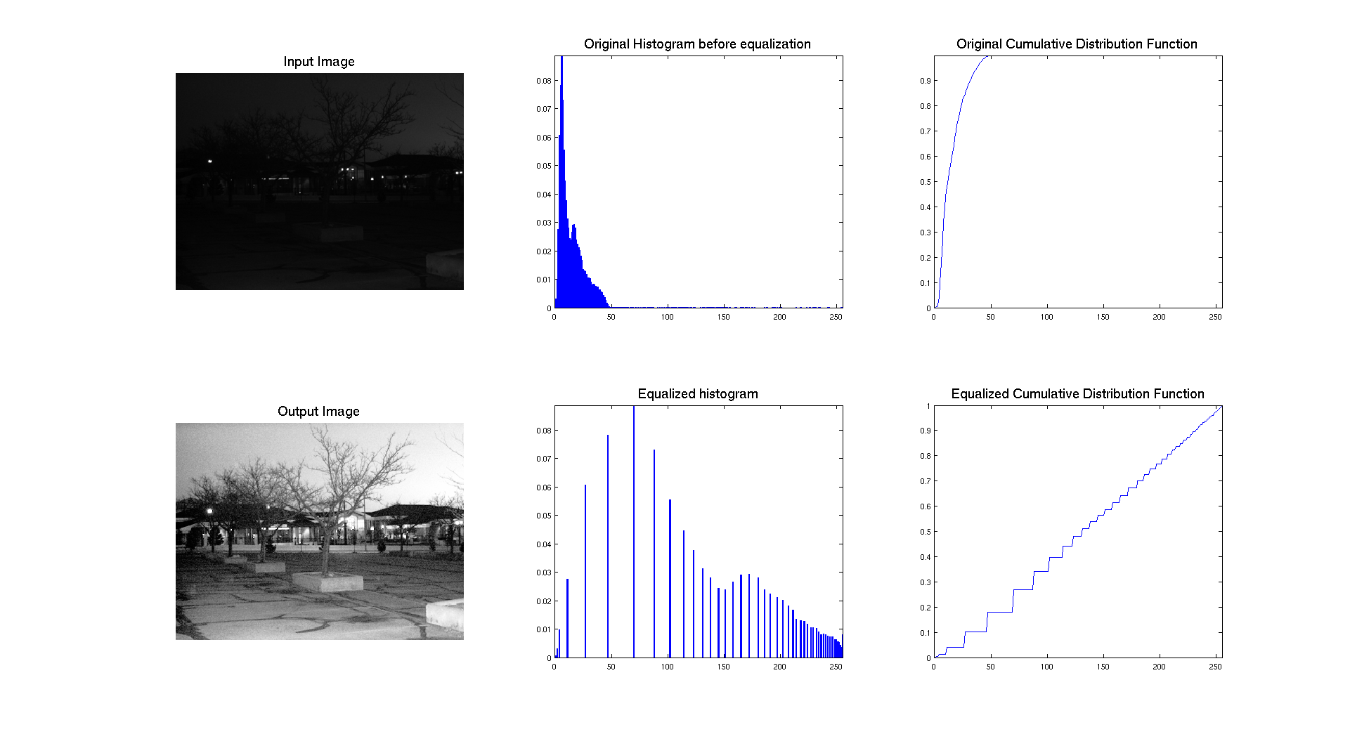
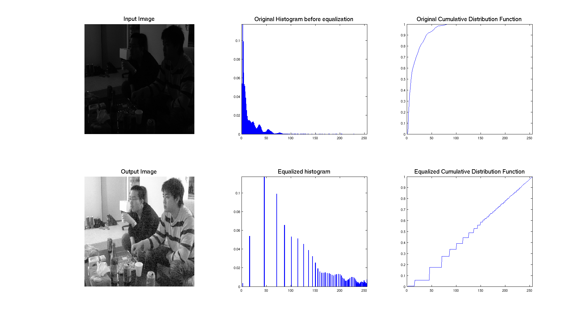
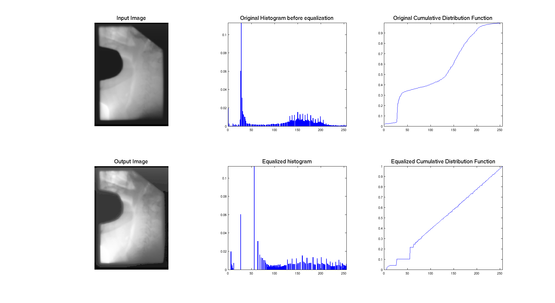
The two previous pictures: university.tif and chang.tif have a similar histogram which in concentrated on the left with a lot of dark intensities. On these images, the histogram equalization is really stretching the histogram and allow us to really see the details of the image that we were not able to see before.
Let's interpret the resulting cumulative distribution. As we can see it's compose of different steps, which approximate a line. The reason why the steps are bigger is because originaly, the histogram was really compressed on the left and the equalization stretched it over the whole range of values. So the higher the peaks are, the higher the step is on the cdf.
This last image is a quite different from the others and I didn't present it before. So as we can see on its histogram, we have a peak of dark gray values that probably represent the background of the image and then a wide range of values on more brighter intensities. So it's pretty logical to have a cumulative density function with such a behavior: a step where the peak is located and then a more smooth evolution to 1 contrary to other images which get close to 1 pretty fast.
So, the cumulative distribution functions looks more like a line because the histogram hasn't been stretch as much as the other images because its original histogram was already distributed on the whole range of intensities. So this is why the result doesn't seem to be changed a lot and the contrast stays quite the same. We can see some more details but this could maybe be enhanced more.
So we can conclude this part that histogram equalization really depends on the initial distribution of intensity levels. If they are concentrated on one side of the histogram, equalization will stretched it to cover the whole range and will enhance contrast. But if the histogram is already distributed over almost the whole range of intensities, equalization will not be as effective because the stretch is not going to be as strong so it's not going to change a lot the intensity distribution.
II: Other images
I decided to run the histogram equalization technique on other images with different types of histogram to see how this is affecting them. Here are the results:
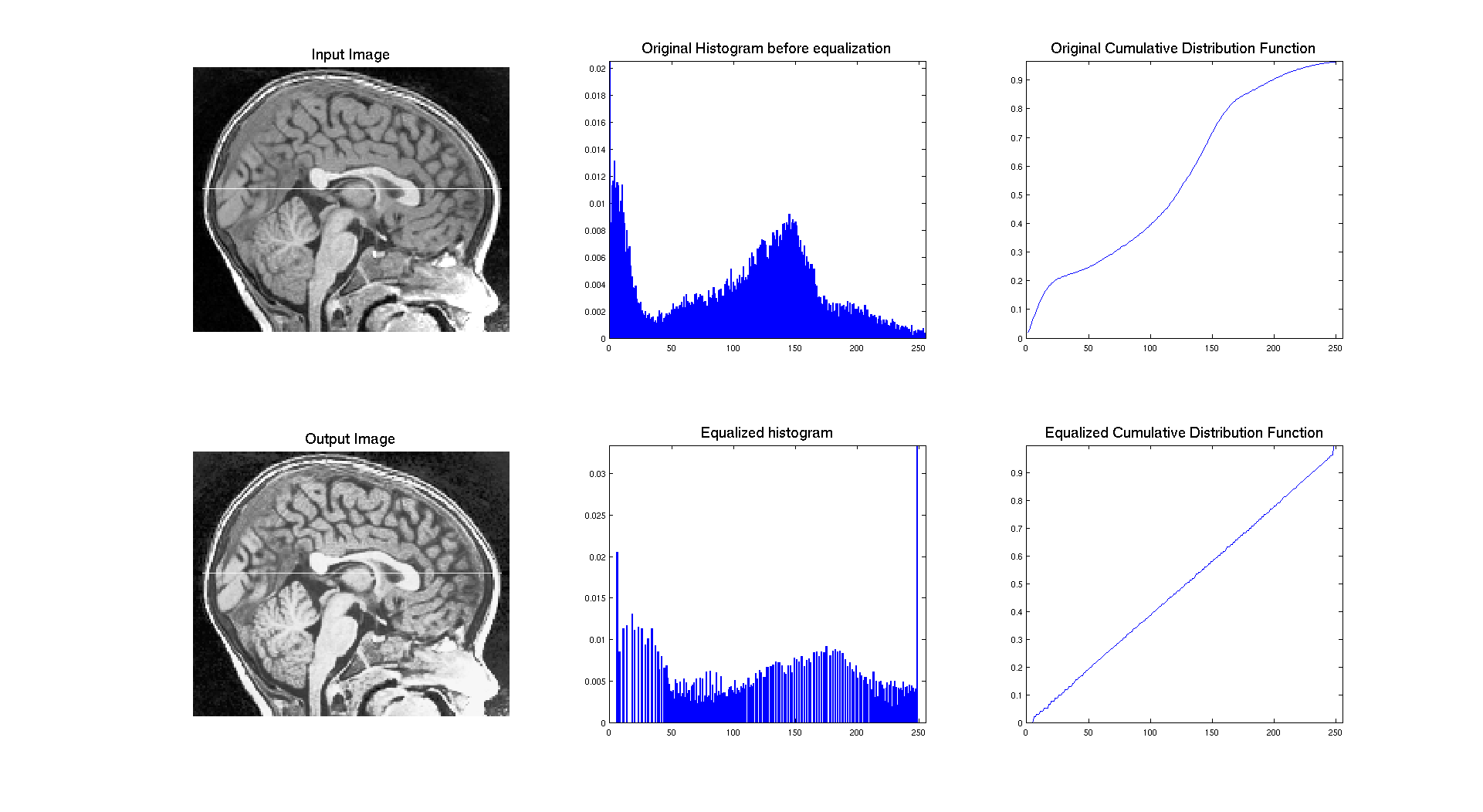
On the previous result, we can see that the input image has an histogram occupying the whole range of gray levels and with a cumulative distribution which is going up really smoothly without big steps. We can see that the result of equalization is here a compression of few levels of the histogram. The image being initially good enough, equalization is not enhancing anything it just makes it brighter by moving the big center peak on the right.
Another interesting thing to test is the opposite thing of what we want. Indeed, if we consider an image where the pdf is already almost uniform, what is going to happen ? To do so, I generated a noise image ( I assume it's white noise (occupying the whole range of level)) and I used it as input of the equalization function.
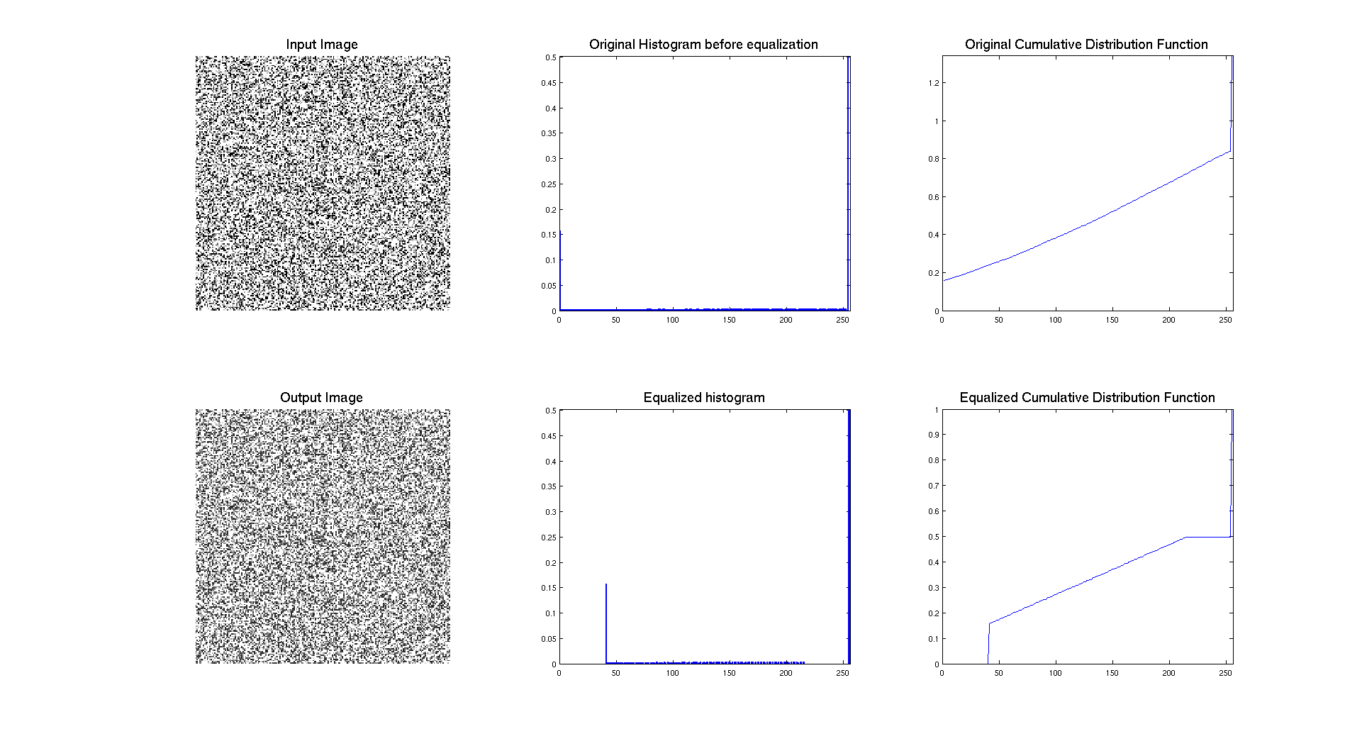
So, here we can see many things, firstly that there is an issue in the display of the cdf which is not ending at the right value. But if we let this aspect we can see that the result of the operation is clearly a compression of level. So two explanations, maybe this issue with the cdf is really screwing things or the equalisation is compressing our histogram. But the contrast is quite the same, so it's in this case really hard to judge the efficiency of the technique in that case. The only thing we can say is that the resulting cdf is no longer linear, which could be explained by the two "dirac" a 0 and 255 which are probably influencing the whole thing. This is indeed due to a programming issue... in the manner to take in account the range of the histogram.
III: Blending
In this part, the idea is to blend two images to get a good compromise between an original image too dark and an equalized image too bright. To do so we are going to use the same pipeline of equalization as before except that the resulting image is going to be a linear blending of the original image and the equalized one according to the following formula:
\[ \text{OutputImg} = \alpha \times \text{EqualizedImg} + (1 - \alpha) \times \text{InputImg} \]
Here is a result when applied to the crowd image, very dark initially and maybe to bright at the end.
We can clearly see that the blending occurred, when looking at the output pdf and cdf, because the cdf is no longer linear. So the idea is to get an intermediate image which will be enhanced but not to much so it does not become too bright. And it seems that it's pretty well working with the blending ratio I choose.
Segmentation by thresholding
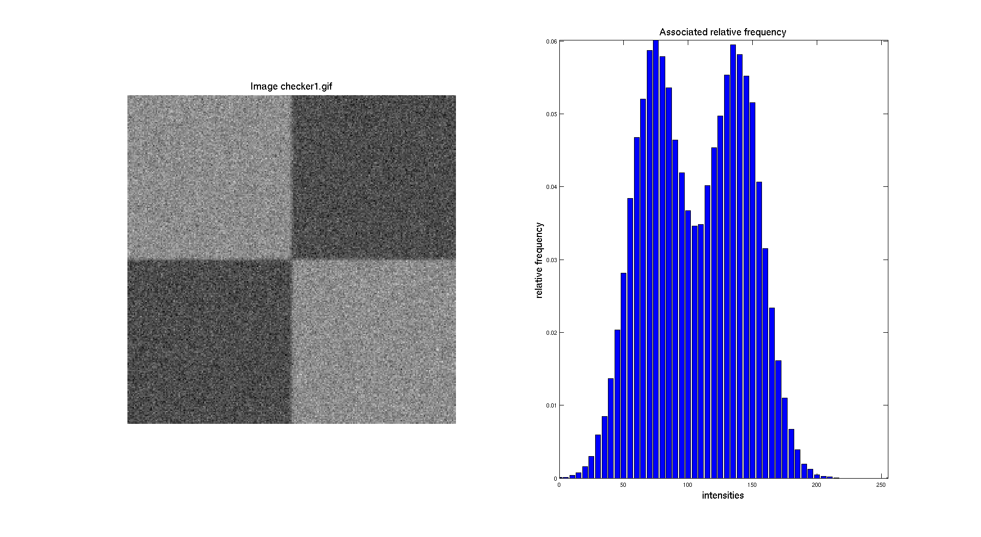
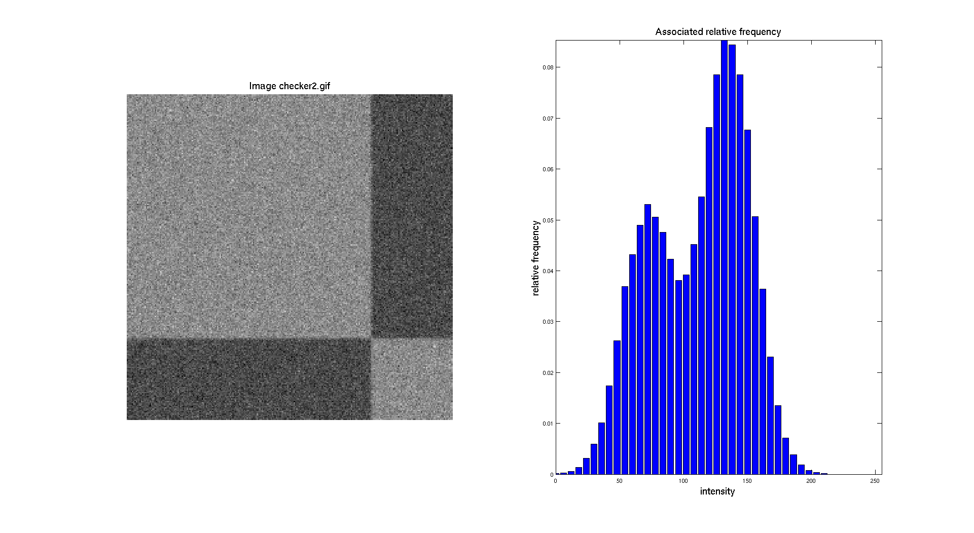
In this part, we are going to work with the following images : two checker board with additional Gaussian noise and the CT scan image. Let's start by displaying the histograms of the two checker board. The gray/black region ratio is not the same on the two images and we can clearly see this aspect while looking at their respective histograms.
I: Checkerboard histograms
The objective here is to be able to perform a segmentation, so to separate distinctly the two regions and create a binary image. To do so, the easiest method to do that is by doing a manual threshold based on the intensity distribution showed in the histogram.
As presented before, I'm in this part implementing the formula presented in the theoretical definitions at the beginning of this report.
II: Thresholding
A: Methods
To be able to segment the image, we need to find a threshold that is representing a good value to separate the two different gray level. Indeed, here the noise is making things a bit harder. To do so, several methods are available, manually select a value, determine an average, use a function.
The first solution as said before, is to chose manually a value that falls exactly in the valley between the two peaks. So we can either read the value on the histogram or use a point clicking operation with the mouse. Either way this is going to be dependent of the user.
The second solution would be probably a bit more accurate, by computing the mean value between the two peaks which will give the exact value. The issue here is if the mean is not an integer, because we will have to either round, ceil or floor it. But this could be more accurate than the manual selection if the noise has the same standard deviation. So we just need here the two original intensity levels before applying noise.
A last solution could be to define a function which will describe the histogram and then run an optimization to find a local minimum lying between the peak. So to do that we can rely on the computation of the first derivative which will be minimum at a local minimum or maximum. This could be implemented of course, but this is not going to be very effective, because the histogram is a discrete structure so we need to have a position described by an integer.
So Here, we will firstly use the first approach to get some initial results and then we will try to implement maybe a better solution.
Then, to threshold images, we need to assign to each value inferior to the threshold an intensity of 0 and if it's higher than the threshold we assign an intensity of 255.
B: Manual Threshold
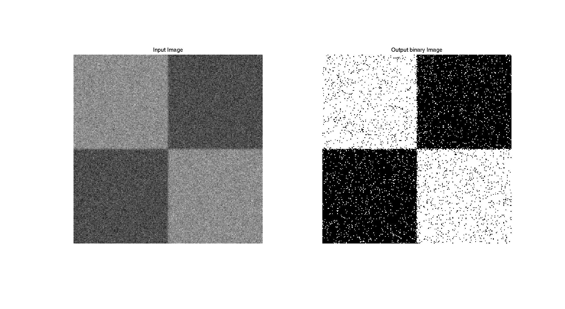
For a first approach, we are going to determine a threshold based on the histogram of the image. We can notice that the minimum of the valley between the two peaks is around 110 for the first checkerboard. So let's look what we obtain if we use this value.
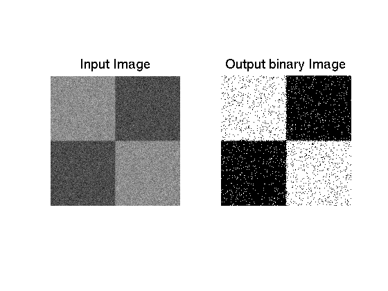
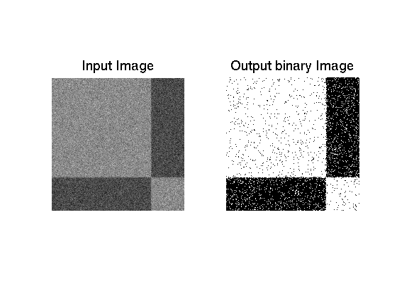
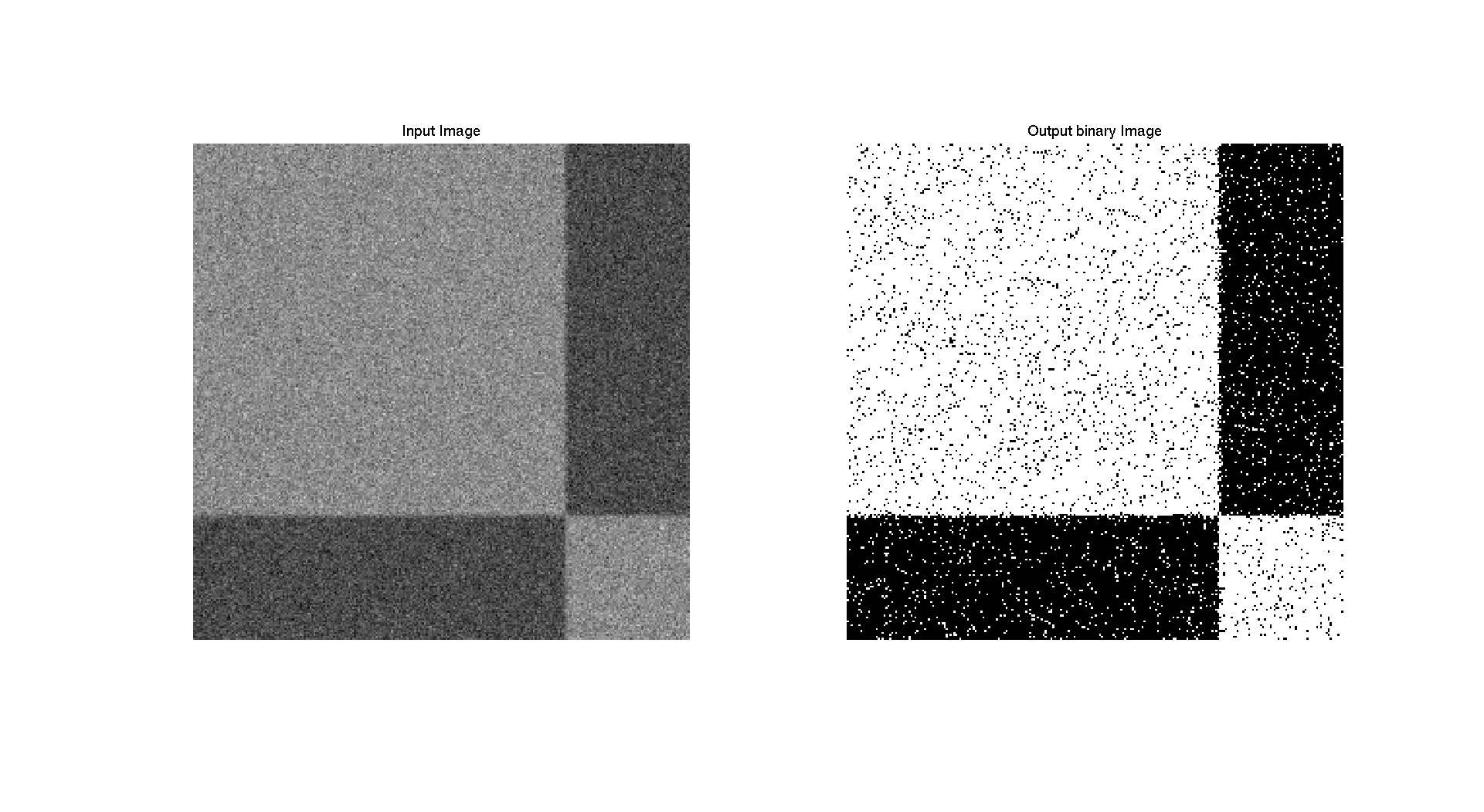
As we can see on the previous image, we can get a fairly good segmentation of the image but because of the noise, we have a certain number of pixel that are associated to the wrong color. These pixels are false positive or false negative and we will discuss this later. This aspect is also present on the second image because there is a noise issue that makes harder the determination of an accurate threshold value.
As we mentioned before, there are two sources of Gaussian noise on this images and it appears that they are overlaying each other. So the idea here is to get more information about these two Gaussian noise distributions.
C: Determination of Gaussian noise characteristics
As presented in section IV of the theoretical definitions, a Gaussian distribution is characterized by two parameters: its mean and its standard deviation. So, to be able to model the two distributions, we need to know these parameters. To determine them, we are going to consider some patches in the image where we compute the mean and the standard deviation. Here are the results we have if we consider two patches of 10x10 pixels in each region of the first checkerboard:
\[\begin{cases} \text{dark area:} \quad \bar{m_1} = 139.2 \quad \sigma_1 = 20.8 \\ \text{bright area:} \quad \bar{m_2} = 77.3 \quad \sigma_2 = 20.2 \end{cases} \]
So, we can plug them into the definition of the Gaussian pdf:
\[ \begin{cases} G_d(x) = \frac{1}{\sqrt{2\pi}\sigma_1}e^{\frac{-(x-\bar{m_1})^2}{2\sigma_{1}^2}} \\ G_l(x) = \frac{1}{\sqrt{2\pi}\sigma_2}e^{\frac{-(x-\bar{m_2})^2}{2\sigma_{2}^2}} \end{cases} \]
Their associated plot is:
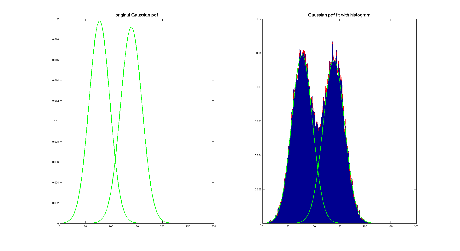
Here, we used a scaling factor to make the pdf fit with the histogram. This scaling factor is 1/2 because of the area covered by each color. Indeed the explanation is easy, each Gaussian pdf has the sum of its density equal to one, so here we want the sum of both densities being equal to one, so we have to scale them according to the amount of pixel of the image they are representing.
We can, of course, do the same with the second checkerboard.
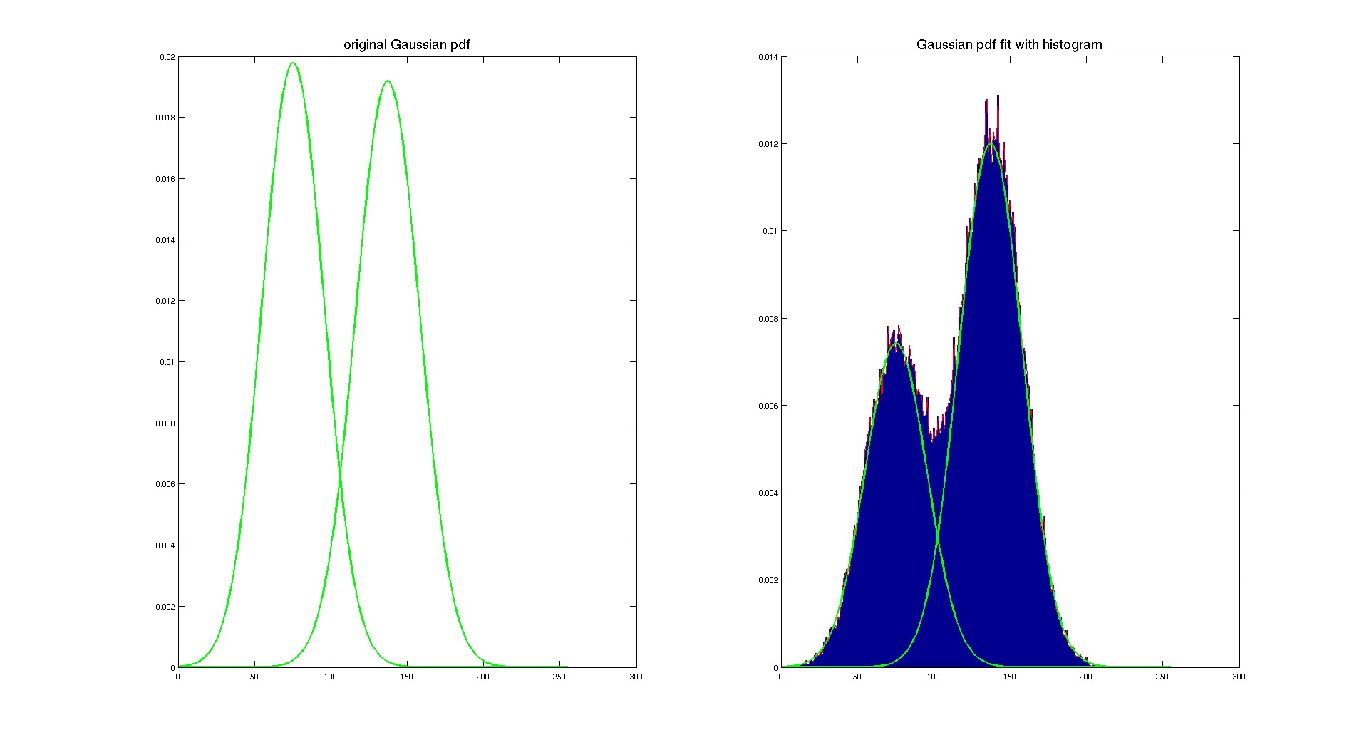
On the previous image, we display the original Gaussian pdf computed using the mean and the standard deviation determined with the patches in both areas. And then by using a scaling factor, we overlay them on the histogram of the image to show that they actually really fit with our original intensity distribution. To determine the scaling factor, we considered that the light gray area is covering 10/16 of the image and the dark gray is covering 6/16.
As we can see on the previous picture, this method is working pretty well, it gives two nice Gaussian distributions which describe our histogram. Of course, both pdf are the same because the only difference between the two checherboard is the area covered by each color. And that's here the only difference between them, because both checkerboard have the same original color and it appears that they are corrupted with the same Gaussian noise.
D: Thresholding based on Gaussian pdf
Once we know the mean and standard deviation of both Gaussian pdf, we can determine a threshold by finding the intersection of the two pdf. To do so we are going to look for a point where the difference between the two curves is really small and this point will be the place where both curves meet and it will be our threshold.
Here are the results for the first checker board where the algorithm gives us a threshold of 108 which is pretty close to the one we used with manual selection. The resulting binary image is close to the previous one.
Regarding the second checkerboard we can make the same observation, we obtain a threshold of 106 which is also quite close from 110 that we chose before.
But there is an important thing to notice, in the previous case, we didn't use a "scaling" factor according to the area of the image associated to each color. We only used the raw Gaussian pdf. So we computed again the threshold introducing this ratio and we got some the following threshold: 108 and 103 for checkerboard 1 and 2 respectively. And the results look a bit better and are closer to the one obtained before. To find which threshold was better we could have substracted the different results to each other to see what was different between them, but it's maybe not the point of this part.
To conclude this part, I think that the method using Gaussian pdf characteristics is pretty accurate and provide a good segmentation which is automatic contrary to the manual selection. But in both case there is a bias due to the overlap of the two distributions:
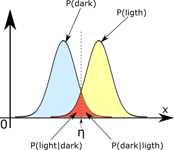
In this case we can clearly see that some pixels are considered bright while they are dark and vice versa. To solve such an issue it exists a solution based on detection and statistics where we can build a model based on both distribution and a Bayesian analysis which could reduce that issue. This solution is providing the optimum thresholding function for a monodimensional problem involving two Gaussian distributions. Due to the complexity of such a thing I just mention it here as a quick conclusion to say that there exists some solutions.
III: CT scan Thresholding
In this last part, we are going to apply the previous method to a medical image in order to extract a bone structure from a CT scan of the head. Here is the histogram of this picture:
To extract the bone structure from this image, we need to segment the image with a high intensity value because the bone is white and other structures are darker. So based on the histogram we have, it seems possible to perform such an operation.
As we did before, we are going to select small patches in the image to get the mean and the standard deviation. But here it's a bit more tricky than before to get accurate patches, this is why on the following plot, the Gaussian distributions are not describing correctly the histogram.
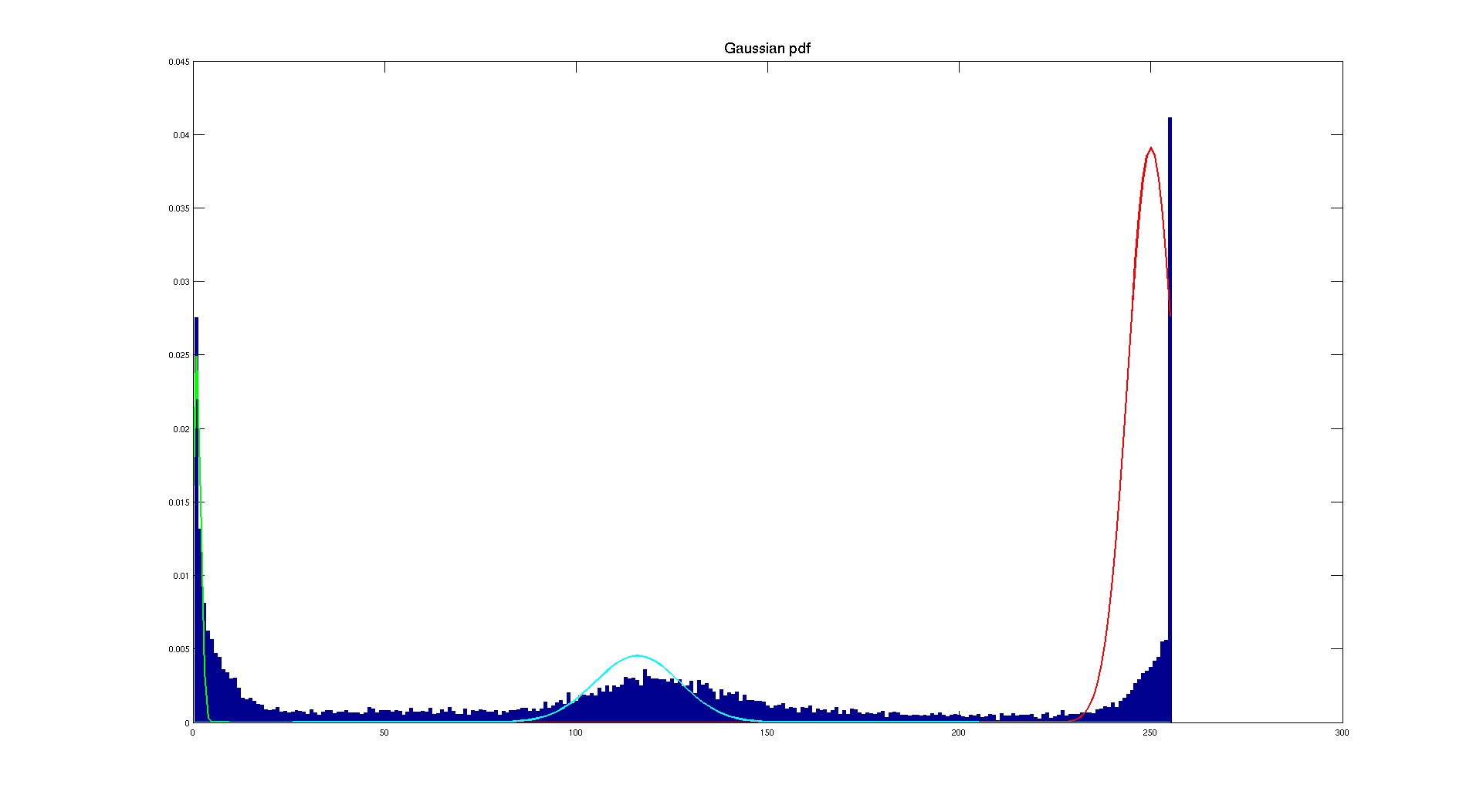
If we play around with patches or define ourselves the average and the standard deviation we can have a better fitting. But this is not the point here because even without we can determine a threshold by looking at the bone Gaussian approximation. Indeed, we can consider a threshold of 230 which will give us the following result:
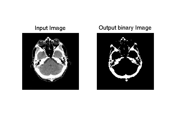
As we can see, the result is quite convincing because we really get the skull. But we could still lower the value and get good results. The idea here is to get only the bone so the risk if we take it to low is to get the skin which also appears white. So there is some possible improvements but the result we have here seems good.
Implementation
I: Histogram function
The function used for this part is defined with the following prototype histogram(Image,nbins,min,max,display) where nbins is the number of bins chosen to perform the histogram, and min and max the two values for the range of the histogram. The display parameter is a Boolean parameter which activate the display of the input image and the associated histogram. It returns a vector containing the relative frequencies associated to the histogram. The core of the function is the computation of the histogram in number of pixels and then in relative frequency respecting the range and the number of bins. Here is the implementation of this part:
for i=1:1:size(InputIm,1)
	     for j=1:1:size(InputIm,2)
		value=InputIm(i,j); %read input image level
		if value >= minvalue && value <= maxvalue
		    for i=1:1:nbins
		        if value <= i*binsize+minvalue && value > (i-1)*binsize+minvalue
			    % original histogram in pixels
		            InputIm_histogram(i)=InputIm_histogram(i)+1;
			    % normalized histogram pdf
		            InputIm_normalized_histogram(i)=InputIm_histogram(i)/resolution;
		        end
		    end
		end
	    end
end
There is a test running before computing the histogram. Indeed, we make sure that the parameters given to the function are correct, so we verify that the number of bins is positive and that the minimum value of the range is inferior to the maximum value.
There is a display parameter, it's a Boolean value used to display the image and its histogram which is performed only if display==1.
Usage:
	%histogram with 100 bins on the full range of levels and without display:
	histo=histogram(Image,100,0,255,0)
	%histogram with 25 bins on a subset of the full range of levels and with display:
	histo=histogram(Image,25,100,200,1)
II: Histogram equalization function
In this part, we are going to rely on the histogram and also on the normalized histogram. To perform this operation, we are going to rely on the function we implemented in the previous part to provide us the normalized histogram.
Then the next step is to compute the associated cumulative distribution function. To do so, we are going to loop on the normalized distribution and add up each time a new probability according to the formula given in section IIIB of the theoretical section.
Once we have the cdf, we are going to "stretch" the histogram to get a "uniform" distribution. To do so, we are going to multiply the cdf by the range of values. See theoretical explanation in section IIIB.
Finally, the last operation to perform is to give to the pixel of the new image the associated new gray level. To do so, we are going to assign to each new pixel the mapped value of the input pixel.
%% Cumulative Distribution function
for i=1:size(InputIm_normalized_histogram,2)
	normalized_cumulsum=normalized_cumulsum+InputIm_normalized_histogram(i)
	normalized_cumulsumvec(i)= normalized_cumulsum
	output(i)=round(normalized_cumulsumvec(i)*levels)  %formula: (L-1)*cdf
end
% Mapping of the original gray level to the new one
for i=1:size(InputIm,1)
	for j=1:size(InputIm,2)
        OutputIm(i,j)=output(InputIm(i,j)+1);
    end
end
To call the function, you need to use the following prototype: OutputIm = histoeq(InputImage,nbins,minvalue,maxvalue,display)
III: Image blending
Here is a quick presentation of the blending function we implemented in the function histoeq_blend(). The idea here is to mix two images to get a good compromise between a too dark image and a too bright image obtained after histogram equalization. So the idea here is clearly to blend them linearly according to what we want to have. We inplemented the function presented earlier in this report and here is the core implementation of it:
for i=1:size(InputIm,1)
    for j=1:size(InputIm,2)
        OutputIm(i,j)=alpha*output(InputIm(i,j)+1)+(1-alpha)*InputIm(i,j);
    end
end
This is a really good way to enhance image contrast but not too much.
IV: Segmentation with histogram function
A: Checkerboard segmentation
In this part, we implemented a pipeline to segment the checkerboard according to a threshold computed from the two Gaussian pdf. So the first step is to define the patches in each area to compute the characteristics of the noise and then be able to plot them.
% define patch 1 in the light grey region
patch1_mean=mean(mean(InputIm(20:30,20:30)))
patch1_std=mean(std(double(InputIm(20:30,20:30))))

% define patch 2 in the dark gray region
patch2_mean=mean(mean(InputIm(210:220,20:30)))
patch2_std=mean(std(double(InputIm(210:220,20:30))))

%% compute Gaussian pdf
for l=0:1:255
    g1(l+1)=(1/(sqrt(2*pi)*patch1_std))*(exp(-0.5*((l-patch1_mean)/patch1_std)^2));
end

for l=0:1:255
    g2(l+1)=(1/(sqrt(2*pi)*patch2_std))*(exp(-0.5*((l-patch2_mean)/patch2_std)^2));
end
Let's explain the computation of the mean and standard deviation. The MATLAB function computing the mean when we give it a 2 dimensional array (our image) is returning an average per column. So we need then to average again the column to get an overall average. This is why we use two times the mean function. This is the same idea for the standard deviation, we compute it for each column and then we average it to have an average standard deviation.
Then we have to find the point where both distribution cross each other. To do so we are looking for the point where their difference is minimal i.e where they are equal. We also consider the ration between dark and bright area to have a better estimation of the threshold.
%% Find the threshold using the two Gaussian distribution
for k=1:255
    if g1(k)*w_ratio-g2(k)*b_ratio<=0.000000001
        threshold=k;
    end
end
The last thing we need to know that we know the threshold is to create the output image by assigning to each pixel it's new value.
%% Applying threshold to create the output image
for i=1:size(InputIm,1)
    for j=1:size(InputIm,2)
        value=InputIm(i,j);
        if value <= threshold
        OutputIm(i,j)=0;
        else
        OutputIm(i,j)=255;
        end
    end
end
We could discuss the choice of considering all values inferior or equal to the threshold but in this case it's not a very influencing factor. Maybe in some specific applications it could be something to take in account but here we can have quite good results.
To call the function, you need to use the following prototype: OutputIm = histoeq(InputImage,nbins,minvalue,maxvalue,display). Which works well with 255 bins, in other cases the display of Gaussian pdf is not going to fit the histogram very well if there are too few bins. The area ratios are automatically adjusted according to which checkerboard you give as input.
B: CT scan segmentation
In this part the implementation is quite similar as before except that we consider 3 patches instead of 2 and that the threshold is manually selected because the Gaussian pdf distributions are helpful to locate an area to threshold but not to automatically determine a specific value.
To call the function, you need to use the following prototype and parameters: threshold_CT(InputImage,threshold,nbins,minvalue,maxvalue,display). Which works well with 255 bins, in other cases the display of Gaussian pdf is not going to fit the histogram very well. The area ratios are automatically adjusted according to which checkerboard you give as input.
Conclusion
To conclude this first project, we can say that we had the opportunity to implement the basic functions of Image Processing. We worked on histograms which are the best tool to understand the distribution of an image intensities.
The part about the equalization showed us how to enhance the contrast of a dark image but also showed us that sometimes if the histogram is already distributed on all the range of levels, the enhancement is not very effective.
The last part involving Gaussian mixture, allows us to determine the characteristics of a Gaussian noise in a image and based on the pdf to determine a value to threshold an image.
There are many aspects involved in this work and on which to add comments and possible solutions. Indeed, there one main things that could be improved. This is the optimum method to get a threshold, the implementation of such a solution is for example Otsu's method to perform thresholding based on minization of the intra class variance. But I didn't have time to implement such a method. But it will be for sure the method to use to get the best possible threshold to obtain a binary image.
Regarding the programming aspect, thanks to MATLAB, we can handle images as matrix which allow us to have a better understanding of the processing. Indeed, the implementation using MATLAB is far from being the fastest and maybe the way I programmed it is far from being the best. But we have this great advantage to just have to manage index and no memory operations or pointers which is a heavier job to do with other programming languages. But If we really want to create a fast and reliable software, solutions exists in C++ and with the ITK library.
This first project was a good way to implement ourselves the major functions used in image processing and that are most of the time performed by image processing software. It allows us to have a better understanding of the global techniques to process an image. The next step being using convolution with filter kernel to create some special features such as blurring or edge detection.