 |
Wei Liu (u0614581)
weiliu@sci.utah.edu
|
With the objective function defined, we use greedy algorithm to find the local minimum of the function. Each point looks for a new position that minimize the energy function, assuming other points fixed. We iterate over all points, and update them together. The procedure is given in algorithm 1.
Normalizing energy functional: To apply a single set of
parameter to different images, the three energy terms need
normalization. ![]() and
and ![]() is normalized by deviding by
the maximal energy in the local neighborhood,
is normalized by deviding by
the maximal energy in the local neighborhood, ![]() is
normalized by
is
normalized by
![]() , where
, where ![]() and
and ![]() is the maximal and minimal gradient magnitude in the local neighborhood.
is the maximal and minimal gradient magnitude in the local neighborhood.
Bonus question: Coarse-to-fine contour: Similar to scale space, we can use a big Gaussian filter to get gradient magnitude map on a higher scale, and run snakes algorithm on this scale. After the snake converges, we use smaller Gaussian kernel to get a finer scale gradient magnitude map, and continue to run snakes, with the previous converged snakes as the initial location. The benefit if this strategy is, at large scale, the snakes easily capture the image gradient magnitude even far away from the shape. At finer scale, the snakes converge to the less smoothed target shape, with higher precision than at coarse scale. Hence this method is both robust to noise, and precise. The following experiments will by default use this strategy unless otherwise stated.
I also note the greedy algorithm's solution is not global optimum. So one need to choose initial landmark points carefully.
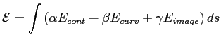
Verify the ![]() term: To ensure that I understand the behavior of each individual energy function, I first only use
term: To ensure that I understand the behavior of each individual energy function, I first only use ![]() and set
and set ![]() and
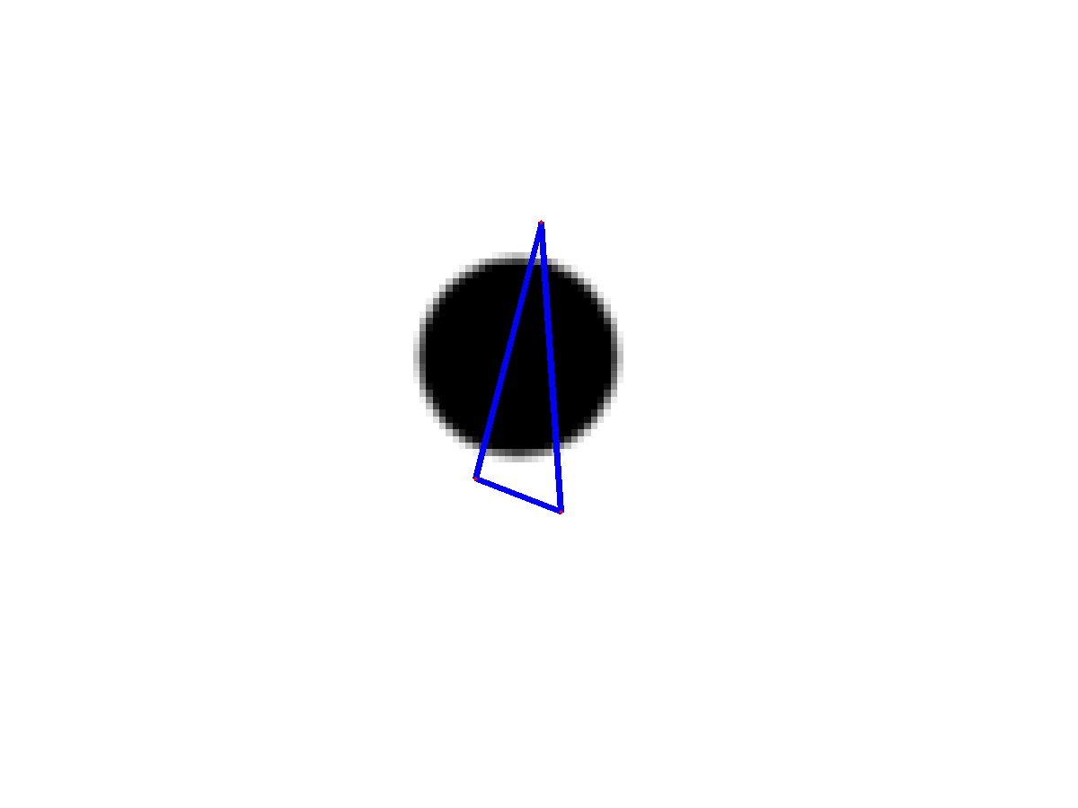
and ![]() to zero. Theoretically, if I just use two points, it will not move by all means. If I use three points, it will ends up with a equilateral triangle, because this gives minimal energy. The experiments confirmed my expectation in figure 1. In this figure I use a circle shape and initialize three points randomly. I see only the
to zero. Theoretically, if I just use two points, it will not move by all means. If I use three points, it will ends up with a equilateral triangle, because this gives minimal energy. The experiments confirmed my expectation in figure 1. In this figure I use a circle shape and initialize three points randomly. I see only the ![]() term force the contour to a equilateral triangle.
term force the contour to a equilateral triangle.
|
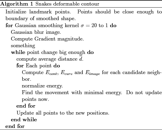
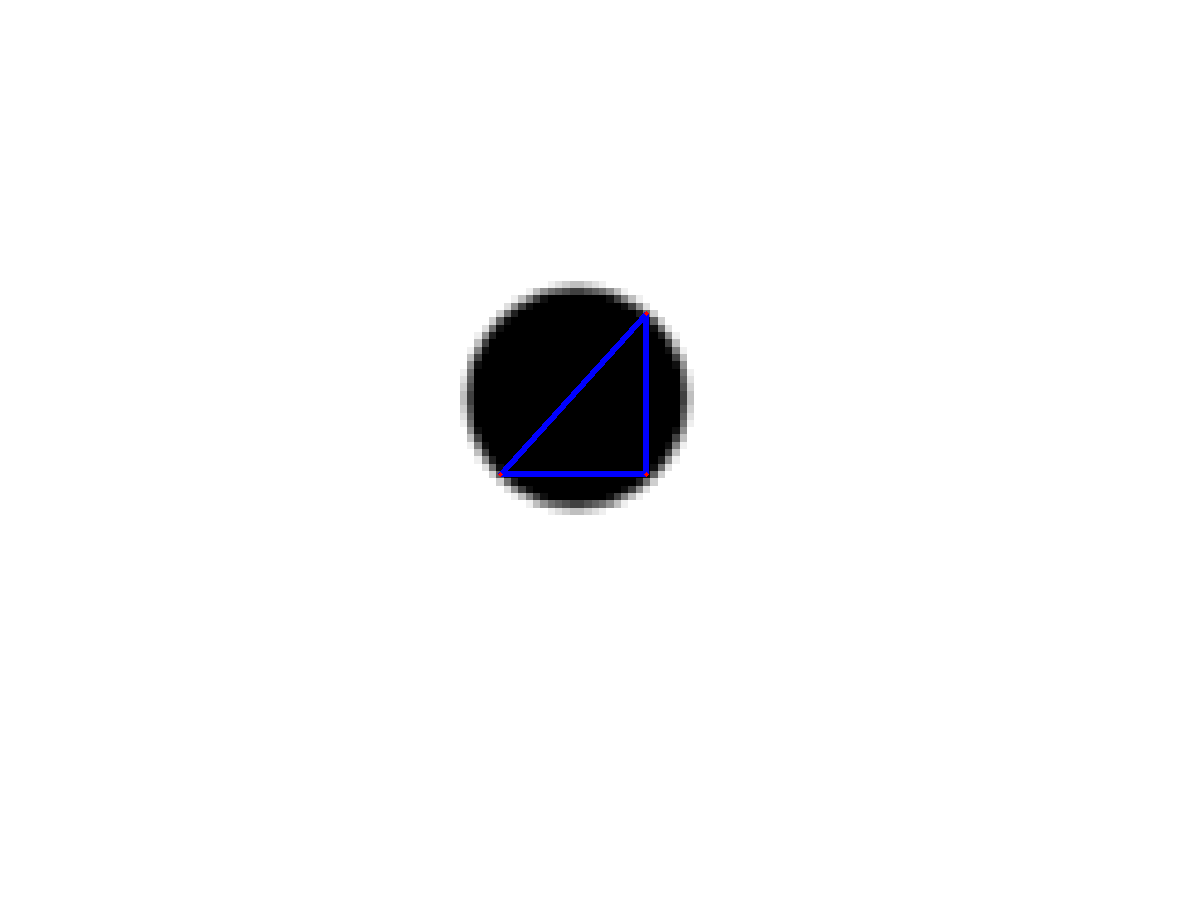
Verify ![]() : Figure 2 shows the results that only
: Figure 2 shows the results that only ![]() are minimized, without considering the internal energy. We see althrough the lanmark points converged to the boundary, they are not evenly spaced. The threee points are all on one half of the contour. The can pose problem, as there may not enough points to represent contour on part of the shape.
are minimized, without considering the internal energy. We see althrough the lanmark points converged to the boundary, they are not evenly spaced. The threee points are all on one half of the contour. The can pose problem, as there may not enough points to represent contour on part of the shape.
|
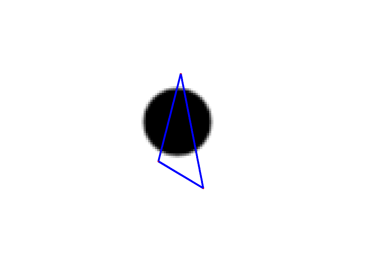
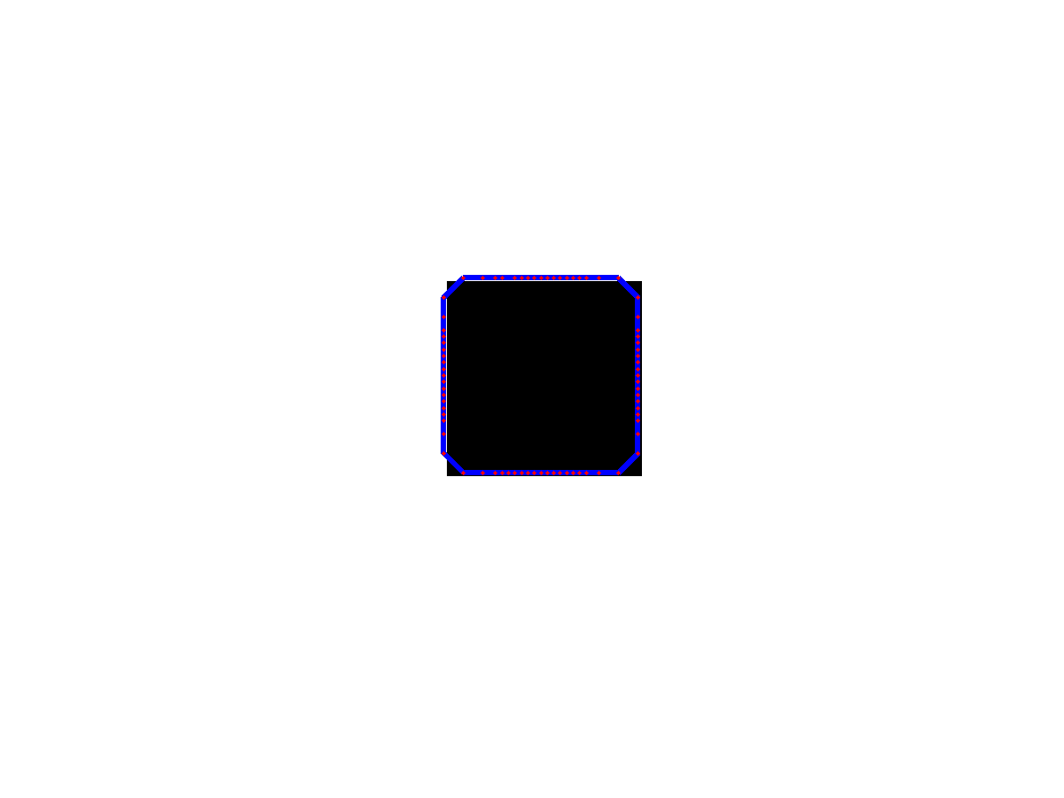
Use both ![]() and
and ![]() : When using both energy terms, we see the points can evenly converge to the shape boundary, as in figure 3.
: When using both energy terms, we see the points can evenly converge to the shape boundary, as in figure 3.


|
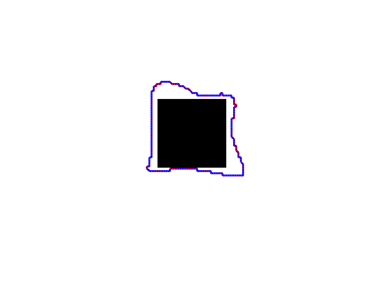
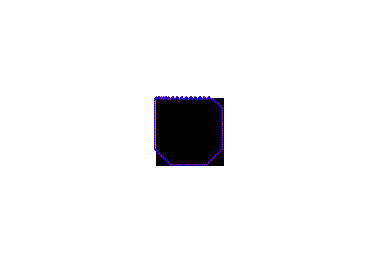
Verify ![]() : To see how
: To see how ![]() works I use a square shape, and run snake with
works I use a square shape, and run snake with ![]() and without
and without ![]() respectively. From figure 4 and 6 I can see without
respectively. From figure 4 and 6 I can see without ![]() the landmark points are able to detect the corners, and with
the landmark points are able to detect the corners, and with ![]() it can not detect it. To say it in another way,
it can not detect it. To say it in another way, ![]() tries to enforce a small curvature contour. sometimes we would want it, because sharp corner sometimes is indicator of noise. but for this square shape we want the snake to find the corner.
tries to enforce a small curvature contour. sometimes we would want it, because sharp corner sometimes is indicator of noise. but for this square shape we want the snake to find the corner.

|
|
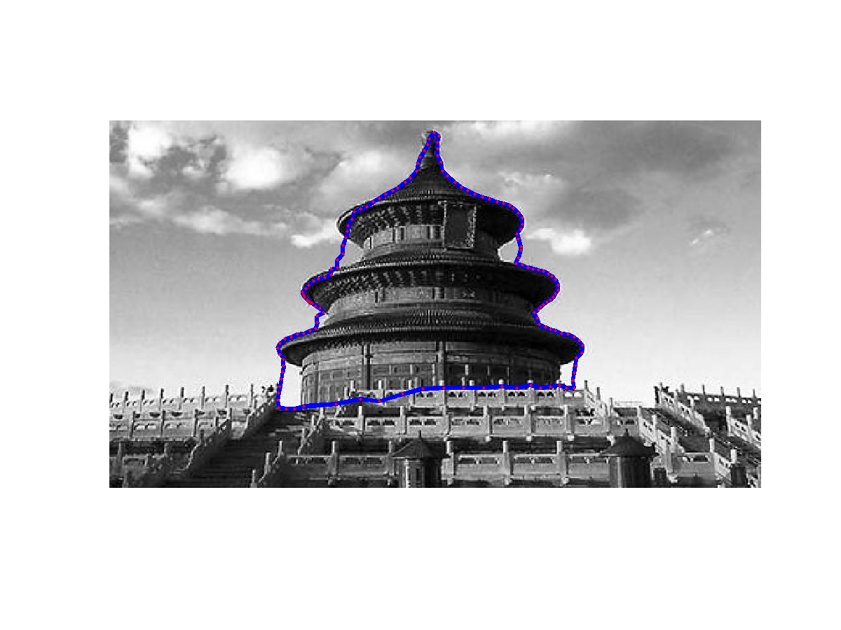
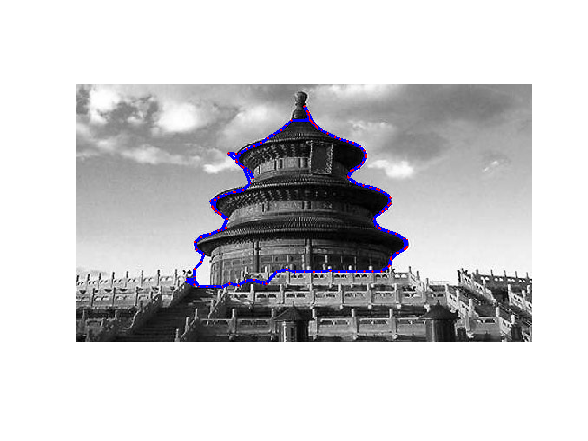
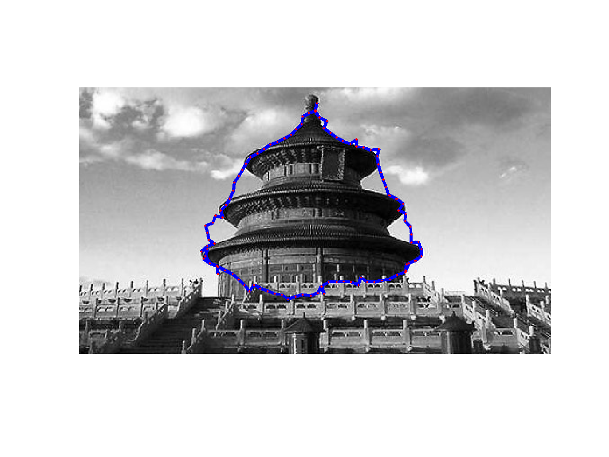
Test on Real data:
|
Turn parameters: I found even I normalized the energy term, different image still need manually ture parameters to get best results. This is probably greedy algorithm is not the best optimization method. Or, we can use other information from image besides the gradient magnitude?
Possible Improvements: Definitely more landmark points have better results. Sometimes adjacent points move to same location, and I wonder if these points can be merged to simplify the following iteration.