Anistropic Diffusion
Wei Liu (u0614581)
weiliu@sci.utah.edu
In this project, I use anisotropic diffusion to smooth and keep the edges unchanged (or even sharpened). Gaussian kernel is used as conductivity function, with its parameter  derived from gradient magnitude we want to keep. Have a brief discussion about the influence of the
  on blurring.
Forward-in-time-centered-space: The explicit formation begin with the heat equation (from West Virginia lecture notes):
And after some approximation the formulation can be written as
where  is the conductivity function, and
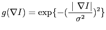
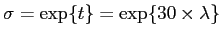
  is the step size on time scale. As required I use Gaussian kernel as the conductivity functionPerona and Malik (1990), i.e.
 |
(2) |
in (1) should be small enough for numerically stability. For four-neighbors,
 , and for eight-neighbors (which is the case in my experiment),
 . I also used
instead of
in the original paper of Perona and Malik (1990) because I think the
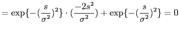
are not equal to
. If we plug into (2), set derivative of
. I also used
instead of
in the original paper of Perona and Malik (1990) because I think the
are not equal to
. If we plug into (2), set derivative of  with respect to
  to zero, to compute the
, we get
to zero, to compute the
, we get
where
is the gradient magnitude,
 . That is to say, if we want to smooth edges whose
  , and sharpen those
  , we need to choose a conductivity kernel (here Gaussian kernel) with
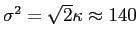 . (not sure about this. Need confirmation)
On the image boundary, I just assume the pixels outside the boundary have same intensity value as the closet pixels on the boundary.
It is worthy noting that for implicit implementation, we need to solve a over-constrained linear equation, and this is more numerically stable with same value of
than explicit formulation.
First, as a warmup we test a simple 'coins' image, as it has a few easily recognized regions (by human vision). I want to keep the edges around the coins, while smooth the details inside the coins. In this experiment, I set the step size in time domain
 . The small step size is because of the eight-neighbor when computing gradient magnitude. The results in figure 1 show the algorithm works pretty well. After difussion. the edges larger than the manual-set threshold (coins' boundary) is smoothed out, and those below threshold (inside coinis) are preserved.
Figure 1:
First row is the original image and the image after 50 iteration of diffusion. Second row is the gradient magnitude map of the image before and after diffusion. Third row is the histogram of the gradient over all pixels. The
value is manually set to 40 as a prior knowledge.
|
Then I use a 'Temple-of-Heaven' image for testing the diffusion under different
. This image is good for testing because it has edges with different gradients. The results is figure 2.
Figure 2:
First row is the original image and its gradient magnitude map. 2nd row to 4th row are the images after diffusion with
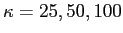 respectively. We can see in 2nd row,only clouds are blurred, also are the fences around the temple. But the temple itself mostly remains. In 3rd row, the fences are further blurred, and the last row even the temple is blurred.
|
to see how more iterations have effects on diffusion, figure 3 has the results. Although this is not a perfect example, we can still see more iteration sharpened the edges above
and smoothed those below
.
Figure:
'Terracotta' image (http://en.wikipedia.org/wiki/Terracotta_Army. First row is the original image and its gradient magnitude map. 2nd row to 5th row are the images after diffusion with iteration
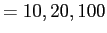 respectively. All the diffusions have same value of
. We can see with more and more iterations, the small textures on the man's body disappeared, but the shape of the warrior, i.e. the edges are unchanged.
respectively. All the diffusions have same value of
. We can see with more and more iterations, the small textures on the man's body disappeared, but the shape of the warrior, i.e. the edges are unchanged.
|
Last we try to compare diffusion by Gaussian convolution in project one, and this explicit formation.
Figure 4:
Comparison between linear smoothing, and non-linear smoothing. Both use Gaussian kernel. First row is original image and gradient. Second row is after anisotropic diffusion with
set to a large enough value, such that it's equal to a linear smoothing. bottom is the linear Gaussian smoothing, i.e. convolution with a Gaussian kernel. The kernel's  is set as
 . Here
can be seen as the time passed in each iteration of diffusion. (comments?)
. Here
can be seen as the time passed in each iteration of diffusion. (comments?)
|
For comparison of linear Gaussian filtering, and non-linear filtering, I noticed linear filtering can be easily implemented in frequency domain because convolution with Gaussian is indeed multiplication in frequency domain. But anisotropic diffusion, as a non-linear smoothing, does not have this nice property. However, is it possible that this anisotropic can be easily implemented in parallel algorithm, and on gpu? I think it is possible, because update of each pixel does not depend on other pixels.
For choosing parameter
: Parameter estimation is a important issue in statistical modeling. Perona and Malik (1990) use a global property of gradient - the histogram to choose
. But I wonder if there is any local statistics we can use to choose
. Say, in a neighborhood, current pixel has large gradient and should remain unchanged, although globally its gradient may be small.
To guarantee numerically stability, the step size at time scale have to be smaller, and this is a downside of anisotropic diffusion. Implicit method is a little better, but still not good enough. Weickert et al. (1998) has a improvement with seems use implicit method.
Anisotropic diffusion is a promising method, if we have good estimation of the
. Besides, it is close to Markov random field, in that both use a 'minimization of energy' concept. It should be able to implement on gpu. This is a quite general method for segmentation (or clustering, depending on how we define the problem). I'll keep this method (and it's spirit) in mind.
After I'm done with the report, I found in my program, I normalized all gradient magnitude to the range of [0, 255], which make it difficult to compare the gradient before and after diffusion. For example, I expect to see some edges are sharpened, but in my results this is not easy to see. Just keep this as notes here.
-
Pietro Perona and Jitendra Malik.
- Scale-space and edge detection using anisotropic diffusion.
IEEE Transactions on Pattern Analysis and Machine
Intelligence, 12 (7): 629-639, 1990.
URL
http://www.scopus.com/inward/record.url?eid=2-s2.0-0025465145&partnerID=40&md5=9f2d3532130bc5f02c5bfd4da5398c91.
-
J. Weickert, B. Romeny, M. A Viergever, et al.
- Efficient and reliable schemes for nonlinear diffusion filtering.
IEEE Transactions on Image Processing, 7
(3): 398–410, 1998.
Wei Liu
2010-02-26

![\includegraphics[width = 0.4\textwidth]{coins.png_init.eps}](img31.png)
![\includegraphics[width = 0.4\textwidth]{coins.png_res.eps}](img32.png)
![\includegraphics[width = 0.4\textwidth]{coins.png_init_grad.eps}](img33.png)
![\includegraphics[width = 0.4\textwidth]{coins.png_final_grad.eps}](img34.png)
![\includegraphics[width = 0.4\textwidth]{coins.png_init_hist.eps}](img35.png)
![\includegraphics[width = 0.4\textwidth]{coins.png_final_hist.eps}](img36.png)
![\includegraphics[width = 0.4\textwidth]{temple2.png_init.eps}](img37.png)
![\includegraphics[width = 0.4\textwidth]{temple2.png_init_grad.eps}](img38.png)
![\includegraphics[width = 0.4\textwidth]{temple2.png_res_25.eps}](img39.png)
![\includegraphics[width = 0.4\textwidth]{temple2.png_final_grad_25.eps}](img40.png)
![\includegraphics[width = 0.4\textwidth]{temple2.png_res_50.eps}](img41.png)
![\includegraphics[width = 0.4\textwidth]{temple2.png_final_grad_50.eps}](img42.png)
![\includegraphics[width = 0.4\textwidth]{temple2.png_res_100.eps}](img43.png)
![\includegraphics[width = 0.4\textwidth]{temple2.png_final_grad_100.eps}](img44.png)
![\includegraphics[width = 0.4\textwidth]{terracotta.png_init.eps}](img45.png)
![\includegraphics[width = 0.4\textwidth]{terracotta.png_init_grad.eps}](img46.png)
![\includegraphics[width = 0.4\textwidth]{terracotta.png_res_it10.eps}](img47.png)
![\includegraphics[width = 0.4\textwidth]{terracotta.png_final_grad_it10.eps}](img48.png)
![\includegraphics[width = 0.4\textwidth]{terracotta.png_res_it20.eps}](img49.png)
![\includegraphics[width = 0.4\textwidth]{terracotta.png_final_grad_it20.eps}](img50.png)
![\includegraphics[width = 0.4\textwidth]{terracotta.png_res_it100.eps}](img51.png)
![\includegraphics[width = 0.4\textwidth]{terracotta.png_final_grad_it100.eps}](img52.png)
![\includegraphics[width = 0.4\textwidth]{annsacks.png_init.eps}](img54.png)
![\includegraphics[width = 0.4\textwidth]{annsacks.png_init_grad.eps}](img55.png)
![\includegraphics[width = 0.4\textwidth]{annsacks.png_res.eps}](img56.png)
![\includegraphics[width = 0.4\textwidth]{annsacks.png_final_grad.eps}](img57.png)
![\includegraphics[width = 0.4\textwidth]{annsacks.png_log.eps}](img58.png)
