Wei Liu
weiliu@sci.utah.edu
The selection of scales are also standard:
![]() , with
, with
![]() . To have a
. To have a ![]() up to 4 is because the first image have a large scale circle.
up to 4 is because the first image have a large scale circle.
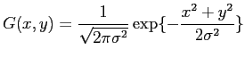
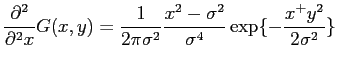
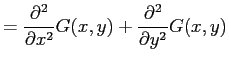
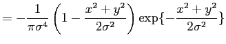
Laplacian filtering: Laplacian filter is usually used to detect edges, as it is able to detect the 'zero-crossing' of second derivative of the signal, which is also the extrema of the first derivative. And that extrema happens at the edges. But because it is very sensitive to noise, good practice is to filter image with a Gaussian filter before Laplacian. Because the convolution is associative, we can convolute the two filter first, then use this LoG filter to convolve with original image. This can save computation. We first define the 2D Gaussian as
 |
(1) |
| (2) |
 |
(3) |
 |
(4) | |
 |
(5) |
    0.0239    0.0460    0.0499    0.0460    0.0239
    0.0460    0.0061   -0.0923    0.0061    0.0460
    0.0499   -0.0923   -0.3182   -0.0923    0.0499
    0.0460    0.0061   -0.0923    0.0061    0.0460
    0.0239    0.0460    0.0499    0.0460    0.0239
Maximum detection strategy: After filtering with LoG at all scales, I have a 3D response ![]() , which the third dim as the scale form
, which the third dim as the scale form ![]() to
to ![]() . To detect the local maximum as candidate of circle center, I search all pixels in all scales. For each pixel, if its response intensity value
. To detect the local maximum as candidate of circle center, I search all pixels in all scales. For each pixel, if its response intensity value ![]() is greater than all its neighbors I'll pick it out as an candidate.
is greater than all its neighbors I'll pick it out as an candidate.
Remove fake candidates that close to each other: Because the candidate circle center may not be at exactly same location with true center, there may be multiple fake responses to same circle. A simple method to detect if two candidate
![]() and
and
![]() is same blob can be
is same blob can be
That is, if the distance between two blobs centers are smaller than the larger circle center (which can be obtained by
![]() ), I'll have to remove one of them that has less response at circle center. by this method, I can remove circles with one half overlapped.
), I'll have to remove one of them that has less response at circle center. by this method, I can remove circles with one half overlapped.
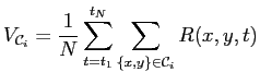
Remove fake candidates by blob volume: I also defined a criteria to remove the blob that are not significant enough. Lindeberg (1993) links the blob in different scales and compare the significance of all blobs by looking at the contrast, spatial extent and lifetime. Here we simplified his method and only look at the mean volume of a blob over all scales.
We informally define the volume of a blob (or a circle in 2D) as the volume of the 3D shape if we regard the response value after filtering as the third dimension. We'll see this is the combination of contrast and spatial extent from the formal definition below
![\includegraphics[width = 0.4\textwidth]{onecircle_blob_vol.eps}](img31.png)
|
We first do test on a simple 'onecircle' image and have the results in 2. The filter works well for this simple image. I also plot the reponse of the circle center over all scales, just to get a glimpse how it looks like. The dynamic filtering at all scales can be found at this GIF image: http://www.sci.utah.edu/~weiliu/class/aip/p1/onecircle.png.gif.
![\includegraphics[width = 0.33\textwidth]{onecircle_bestscale.eps}](img32.png)
![\includegraphics[width = 0.33\textwidth]{onecircle.png_resp.eps}](img33.png)
![\includegraphics[width = 0.33\textwidth]{onecircle.png.eps}](img34.png)
|
We then move to the multiple circle in the second image. In multiple circle detection results (fig. 3), we notice: Two blob close to each other have interference in higher scale, because they tend to merge and give inaccurate circle center. We can see a blue color circle close to the right plot's center-left region, and the algorithm did not detect the center accurately. I did not deal with this issue in this project, but am aware of one solution Lindeberg (1994) that consider the 'split' or 'merge' of two blobs in adjacent scales.
The dynamic scale-space filtering results can be found at http://www.sci.utah.edu/~weiliu/class/aip/p1/scalespaceTest.png.gif.
![\includegraphics[width = 0.4\textwidth]{scalespaceTest.png_resp.eps}](img35.png)
![\includegraphics[width = 0.4\textwidth]{scalespaceTest.png.eps}](img36.png)
|
For 'sunflower2' image, the results is fig. 4. For this real-world image, the algorithm detected some local maxima as circle center, while these are actually not real circle (from human vision). By using the threshold of (7), I only choose those candidate circle center with big average blob volume as final results. The threshold of the average blob volume is set to ![]() , which is rather ad-hoc procedure.
, which is rather ad-hoc procedure.
From the results of fig. 4 we see the false positive mostly come from locations much like real circle. Some triangle, and square shaped region, are detected as circles. To further improve the algorithm, I think we can look at not only the peak (and volume) of the blob, but also the shape of the blob. Since we know the shape of a circle blob after Laplacian filtering, we can compare the candidate blob's shape with ideal shape, and hopefully will remove fake circles originated from other shapes (triangle, square, etc.)
![\includegraphics[width = 0.4\textwidth]{sunflower2.png_resp.eps}](img38.png)
![\includegraphics[width = 0.4\textwidth]{sunflower2.png.eps}](img39.png)
|
The forth image have detection results in fig. 5. We can see because around the arm and chest of the baby, there is a shape that has almost closed boundary and looks very much like a circle. The algorithm ends up detecting it as a circle, hence a false positive. But the false positive circles around the baby's head is not what I expected.
![\includegraphics[width = 0.4\textwidth]{sunflower3.png_resp.eps}](img40.png)
![\includegraphics[width = 0.4\textwidth]{sunflower3.png.eps}](img41.png)
|
Below is some tests on images of myself. See fig. 6 and 7.
![\includegraphics[width = 0.4\textwidth]{penny-round-mix.jpg.eps}](img44.png)
![\includegraphics[width = 0.4\textwidth]{penny2.jpg.eps}](img45.png)
|
![\includegraphics[width = 0.4\textwidth]{planet_my.png.eps}](img42.png)
![\includegraphics[width = 0.4\textwidth]{planet2.jpg.eps}](img43.png)