|
In this section, we highlight the latest additions to map3d in the (vain?) hope that people will read at least this much of the manual and be able to quickly make use of the latest and greatest that the program offers.
This is the fourth version of the ``new'' map3d with a GTK-based GUI. We are getting very very very close to the complete functionality of the old GL based version and have gone well beyond it in some features, especially the user interface. This is a ``dot'' release but is not a minor release for it contains some important new features and the usual set of bug fixes.
Some of the specific additions that you should notice over previous versions include:
A small sampler of things that are in the works:
g
This document describes the function and usage of versionversion of the program map3d, a scientific visualization application originally developed at the Nora Eccles Harrison Cardiovascular Research and Training (CVRTI) and now under continued development and maintenance at the Scientific Computing and Imaging Institute (SCI) at the University of Utah. The original purpose of the program was to interactively view scalar fields of electric potentials from measurements and simulations in cardiac electrophysiology. Its present utility is much broader but continues to focus on viewing three-dimensional distributions of scalar values associated with an underlying geometry consisting of node points joined into surface or volume meshes.
map3d has been the topic of some papers [1,2,3,4] and a technical report [5] and we'd love it if you would reference at least one of them (perhaps [3] or [4] are the easiest ones to get copies of) as well as this manual when you publish results using it. There have been many many more papers that use map3d and the list keeps growing.[3,4,5,6,7,8,9,10,11,12,13,14,15,16,17,18,19,20,21,22,23,24,25,26,27,28,29,30]
One of the big changes in version 6.3 is that we are now completely open source. People can download not only the executable but also the complete source code for the program. Please note that we do not have a good way yet to incorporate changes people outside our little group make to the program. If you do wish to change and then contribute back, please let us know as soon as possible and we can try and coordinate as best we can. Of obvious interest is when someone ports map3d to another platform--please let us know about this and we can add it to the list and release it with the rest.
The history of map3d goes back to 1990 and the first few hundred lines of code were the product of a few hours work by Mike Matheson, an inspired visualization specialist, now with SGI in Salt Lake City. This was my introduction to GL and C and this program became my personal sand box to play in. Along the way, Phil Ershler made valuable contributions in figuring out the magic of Formslib for some user interface controls and developing with me graphicsio, the geometry and data file library that supports map3d. Ted Dustman has recently taken up maintenance and extensions of graphicsio and remains my main man when I need programming lessons.
This is one in a series of ``new'' versions of map3d, the series (labeled 5.x or above) that marks the move from GL to OpenGL library and thus to becoming truly portable. In fact, we call the old one map3dGL now to indicate its links to SGI's original GL library. We seem permanently stuck in the middle of this big conversion project, moving support to OpenGL and adding lots of power as we convert functionality. The reason for the version 6.x, was the move to gtk as the GUI library with which we create all the dialog and display elements of the program. This move has allowed us to extend dramatically the set of dialog boxes map3d offers and this newest version 6.3 contains many examples.
There are some people who have been instrumental in the process and deserve special mention. Chris Moulding is a graphics programmer and general software whiz who surveyed my sand box architecture, pulled together the essential walls, created new ways to make rooms, and still left lots of the sand box around so we could continue to play. From version 5.2 onward, Bryan Worthen replaced Chris and really has found the spirit of map3d. Bryan has become the main driving force behind the actual work of coding and fixing. He strayed off to some other project for a while, but never lost his love for map3d; we are really pleased that he has returned to pick up the torch again. Most recently, J.R. Blackham has joined the team while still an undergraduate in Computer Science at Utah. Jeroen Stinstra is my super-postdoc, helpful in more ways than I knew I even needed and full of inventive ideas. He has created the support for MATLAB that we use in map3d (and the SCIRun project) and is best bug-catcher I know.
The largest thanks must go to the users of map3d, who provided the real inspiration and identified the needs and opportunities of such a program. Among the most supportive and helpful are Bruno Taccardi, Bonnie Punske, and Bob Lux, all colleagues of mine at the CVRTI. Dana Brooks and his students from Northeastern University are also regular users who have provided many suggestions and great enthusiasm. Also invaluable in the constant improvement of the program are my post docs, Jeroen Stinstra, and graduate student Quan Ni, Rich Kuenzler, Bulent Yilmaz, Bruce Hopenfeld, Shibaji Shome, Lucas Lorenzo, Andrew Shafer, and Zoar Englemann. They give me new energy every day and remind me why I am a professor. Notable new additions to the family are Randy Thomas from Universite d'Evry Val d'Essonne in Evry, France. The great thing about Randy is that he used map3d to visualize concentrations of ions in his simulation of the nephron! Also, Ed Ciaccio from Columbia University has become a big user and even takes it to his classes.
The first user and long-time collaborator and friend was Chris Johnson and this new version of map3d is possible because of the success he and I have had in creating the SCI Institute and specifically the NIH/NCRR Center for Geometric Modeling, Simulation, and Visualization in Bioelectric Field Problems (www.sci.utah.edu/ncrr).
We gratefully acknowledge the financial support that has come from the NIH, National Center for Research Resources (NCRR) the Nora Eccles Treadwell Foundation, and the University of Utah, which provides us with space and materials to create this sand box. The Nora Eccles Treadwell Foundation has also provided support for the development of map3d and the huge pile of data we have used it to analyze.
Rob MacLeod, May 19, 2005.
The terms of the license agreement under which we release map3d are simple and as follows:
Permission is hereby granted, free of charge, to any person obtaining a copy of this software and associated documentation files (the ``Software''), to deal in the Software without restriction, including without limitation the rights to use, copy, modify, merge, publish, distribute, sublicense, and/or sell copies of the Software, and to permit persons to whom the Software is furnished to do so, subject to the following conditions:
R.S. MacLeod and C.R. Johnson. Map3d: Interactive scientific visualization for bioengineering data. In IEEE Engineering in Medicine and Biology Society 15th Annual International Conference, pages 30-31, IEEE Press, 1993.
THE SOFTWARE IS PROVIDED ``AS IS'', WITHOUT WARRANTY OF ANY KIND, EXPRESS OR IMPLIED, INCLUDING BUT NOT LIMITED TO THE WARRANTIES OF MERCHANTABILITY, FITNESS FOR A PARTICULAR PURPOSE AND NONINFRINGEMENT. IN NO EVENT SHALL THE AUTHORS OR COPYRIGHT HOLDERS BE LIABLE FOR ANY CLAIM, DAMAGES OR OTHER LIABILITY, WHETHER IN AN ACTION OF CONTRACT, TORT OR OTHERWISE, ARISING FROM, OUT OF OR IN CONNECTION WITH THE SOFTWARE OR THE USE OR OTHER DEALINGS IN THE SOFTWARE.
map3d incorporates the functionality of several external libraries. They are:
We use GTK and GtkGLExt to interface with the window manager to give us windows with OpenGL capability, as well as giving us widgets we need for interactive control. We use PNG and JpegLib to be able to save .png and .jpg images of map3d. All four of these libraries are covered by the GNU LGPL, which is included in the distribution of map3d.
As of version 6.3, we also release internal libraries under the same license as above for the rest of map3d.
map3d is written in standard C/C++ and uses the OpenGL and GTK+ libraries, both choices made to ensure broad portability of the program.
| Requirements for all systems. | |
| OpenGL libraries (GL and GLU) | version 1.1 + 1 |
| OpenGL/window interface library (GLX) | |
| GTK+ libraries and dependencies | version 2.0+ |
| Requirements | |
| Operating System | kernel 2.2.x |
| Architecture | i386 (+ maybe PPC) |
| Applications Binary Interface | libc2.1 |
| Recommendations | |
| Window system | XFree86 version 4.0 + |
| Hardware | 3D graphics card (nVidia, 3dfx, ati) |
| 128 MB main memory | |
| Requirements | |
| Operating System | W2K/NT4.0/9x |
| Architecture | i386 |
| Applications Binary Interface | win32 |
| Recommendations | |
| Hardware | 3D graphics card (nVidia, 3dfx, ati) |
| 128 MB main memory | |
| Requirements | |
| Operating System | Mac OS 10.3(Panther) |
| Architecture | PPC |
| Recommendations | |
| Hardware | 3D graphics card (nVidia, 3dfx, ati) |
| 256 MB main memory | |
| Requirements | |
| Operating System | Irix 6.5+ |
| Architecture | mips3 or mips4 (maybe mips2) |
| Applications Binary Interface | n32 or 64 |
| Recommendations | |
| Hardware | Texture mapping hardware |
| 128 MB main memory | |
Unfortunately, with our move to GTK+ for window support, it is not as easy as past versions, which required just the download of an executable. We hope (in vain, perhaps) to be able to do that again in the future, but for now we will attempt to make installation as easy as we can. Simplified instructions will be in a README file which comes with each package, and are also listed below:
To download the software, use this URL www.sci.utah.edu/software/map3d.html, and click on the ``Download'' button. You'll need to sign into the SCI archive. For each of the installation instructions below, you can grab those file from this page.
To test the installation, use the test files that accompany this distribution. Each has some script files included that show how to call and execute map3d.
The Linux installation is relatively straightforward. You'll need to download map3d's dependencies, then download map3d itself.
There are two phases to this part. First we need to get GTK+ and its dependencies. The easiest way to do this is from your distribution's installation CDs, or you can download the RPMs at www.rpmfind.net.
To get the dependencies from your distribution, run the Package Manager (Add/Remove Applications, configure-packages or something of that sort). Search for gtk, and install gtk2 (if you can't find that directly, then installing the gnome environment will take care of it).
To get the dependencies from the internet, navigate your favorite browser to http://www.rpmfind.net, and search for gtk-2.0. Try to find one that matches your distribution (redhat, mandrake, etc.). We directly support development for gtk2-2.2.1 and gtk2-2.0.6, so if you can find one of these that would be encouraged.
The next part is to download gtkglext, the library that supports OpenGL for
GTK widgets. As of this release, this is not standard in most
distributions. If your GTK version is 2.0.6 or 2.2.1 (you can find out by
looking at gtkversion.h which will be where you installed gtk
(normally /usr/include/gtk-2.0/gtk/gtkversion.h), and look for
GTK_MAJOR_VERSION, GTK_MINOR_VERSION, and
GTK_MICRO_VERSION. There will be numbers on the same lines as each
of these, and if you put them together it will be something like 2.2.1).
If you are using one of these versions download
gtkglext-linux-2.2.1.tar.gz or gtkglext-linux-2.0.6.tar.gz from
the map3d download page
and follow these
instructions:
    cd <download directory>
    gunzip gtkglext-linux-<version>.tar.gz
    tar xf gtkglext-linux-<version>.tar
    cp libgtkglext-x11-1.0.so.0 /usr/local/lib
    cp libgdkglext-x11-1.0.so.0 /usr/local/lib
You can copy them to some directory other than /usr/local/lib if you wish.
If this doesn't work, you will need to download the gtkglext source and compile it yourself (don't worry--if your gtk is properly set up, this will be very easy). Download the sources from Source Forge http://sourceforge.net/projects/gtkglext and follow these instructions:
    cd <download directory>
    gunzip gtkglext-1.0.6.tar.gz
    tar xf gtkglext-1.0.6.tar
    cd gtkglext-1.0.6
    configure
    make
    make install
If you don't want these to end up in /usr/local/lib, you need to
configure --prefix=<dir>
where dir is where to put the libraries.
Download the map3d-6.2-linux.tar.gz file from the map3d() download page and unzip it to a directory of your choice. We will call that RUN-DIR. This is the directory from which you will run map3d.
To run map3d, you will need to make sure that all the libraries are in
your LD_LIBRARY_PATH environment variable. For this we will assume
that your gtk libraries are in /usr/lib and your gtkglext
libraries are in /usr/local/lib. Do the following:
tcsh users:
setenv LD_LIBRARY_PATH /usr/local/lib:$LD_LIBRARY_PATHor
export LD_LIBRARY_PATH=/usr/local/lib:$LD_LIBRARY_PATH
you might want to put this line in your .cshrc or .profile file to avoid having to run this multiple times.
The Windows installation is relatively straightforward. You'll need to download map3d's dependencies, then download map3d itself.
Download the map3d-win-environment.zip file from the map3d
download page
and unzip (using winzip,
native windows xp zip file browser, or another windows zip program) it into a location
of your choice - we will call that INSTALL-DIR. It will create a
directory called INSTALL-DIR\map3d.
Add INSTALL-DIR\map3d\lib to your path. To do this, open the
Control Panel, select System, and click on the `Advanced' tab on the top of
the screen. Click on the Environment Variables button. You should see a
variable called Path or PATH in the System Variables section. Click on it,
and select Edit. Go to the end of the line, add a semi-colon (;) and type
INSTALL-DIR\map3d\lib.
There is an executable of map3d in the environment directory. We have also placed an executable here to facilitate future downloads, so you only have to download the environment once. If you wish, download the map3d-6.2-windows.zip file from the map3d download page and unzip it to a directory of your choice. We will call that RUN-DIR. This is the directory from which you will run map3d.
The Mac OS X installation is relatively straightforward. You'll need to download map3d's dependencies, then download map3d itself.
Map3d requires the gtk+2 and gtkglext libraries. You can easily install these libraries using fink.
If you do not currently have fink installed on your system you will need to go to http://fink.sourceforge.net and follow the instructions on how to install it and the gtk+2 and gtkglext libraries.
Download the map3d-6.2-mac.tar.gz file from the map3d download page and unzip it to a directory of your choice. We will call that RUN-DIR. This is the directory from which you will run map3d.
The SGI installation is relatively straightforward. You'll need to download map3d's dependencies, then download map3d itself.
fw_gtk2+ (make
sure you don't select fw_gtk+). Submit the query. You should see a
list similar to this:
  fw_atk [relnotes] [prereqs] [install]
  fw_expat [relnotes] [prereqs] [install]
  fw_freetype2 [relnotes] [prereqs] [install]
  fw_gettext [relnotes] [prereqs] [install]
  fw_glib2 [relnotes] [prereqs] [install]
  fw_libjpeg [relnotes] [prereqs] [install]
  fw_libpng [relnotes] [prereqs] [install]
  fw_libz [relnotes] [prereqs] [install]
  fw_pango [relnotes] [prereqs] [install]
  fw_tiff [relnotes] [prereqs] [install]
To install them, click on the install link one by one (and follow the instructions in the dialog boxes).
IMPORTANT - when you install libz - it will mention something about a security library being removed. When you install libz, allow it to do this. On the subsequent libraries, it will mention that the security package conflicts with libz, on these packages, have it continue without installing the security package.
Install them in the order:
    gettext
    expat
    freetype2
    atk
    glib2
    pango
    libjpeg
    libtiff
    libz
    libpng
After you've done all of these, click on the alphabetical link, and click on
the install buton that corresponds to libgtk2+-2.0.6.
If for some reason, the prereq calculator isn't there or isn't working, go to the alphabetical index and install the above in the order specified.
The next part is to download gtkglext, the library that supports OpenGL for
GTK widgets. If your GTK version is 2.0.6 (you can find out by looking at
gtkversion.h which will be where you installed gtk (normally
/usr/freeware/include/gtk-2.0/gtk/gtkversion.h), and look for
GTK_MAJOR_VERSION, GTK_MINOR_VERSION, and
GTK_MICRO_VERSION. There will be numbers on the same lines as each
of these, and if you put them together it will be something like 2.0.6).
If you are using this version download gtkglext-sgi.tar.gz from
the map3d download page
http://www.sci.utah.edu/software/map3d.html
and follow these
instructions:
    cd <download directory>
    gunzip gtkglext-sgi.tar.gz
    tar xf gtkglext-sgi.tar
    cp libgtkglext-x11-1.0.so.0 /usr/local/lib
    cp libgdkglext-x11-1.0.so.0 /usr/local/lib
You can copy them to some directory other than /usr/local/lib if you wish.
If this doesn't work, you will need to download the gtkglext source and compile it yourself (don't worry--if your gtk is properly set up, this will be very easy). Download the sources from Source Forge http://sourceforge.net/projects/gtkglext and follow these instructions:
    cd <download directory>
    gunzip gtkglext-1.0.6.tar.gz
    tar xf gtkglext-1.0.6.tar
    cd gtkglext-1.0.6
    configure
    make
    make install
If you don't want these to end up in /usr/local/lib, you need to
configure --prefix=<dir>
where dir is where you want to put the libraries (The libraries will be in dir/lib).
Download the map3d-6.2-irix.tar.gz file from the map3d download page and unzip it to a directory of your choice. We will call that RUN-DIR. This is the directory from which you will run map3d.
To run map3d, you will need to make sure that all the libraries are in your LD_LIBRARY_PATH environment variable. For this we will assume that your gtk libraries are in /usr/freeware/lib32 and your gtkglext libraries are in /usr/local/lib. Do the following:
    tcsh users:
    setenv LD_LIBRARY_PATH /usr/freeware/lib32:/usr/local/lib:$LD_LIBRARY_PATH
or
bash users:
export LD_LIBRARY_PATH=/usr/freeware/lib32:/usr/local/lib:$LD_LIBRARY_PATH
you might want to put this line in your .cshrc or
.profile file to avoid having to run this multiple times.
We have tried to make installing map3d from source as simple as possible. There are four steps:
If you are running on a different system, you will probably need to download and install these on your own; please refer to GTK website and GtkGLExt website.
You should not have to change much in order to get map3d to compile. MatlabIO (one of map3d's dependents) needs to know where ZLIB is (required, and should be installed after completing the previous section), and map3d needs to know where gtk is. The included files show samples of how this is to be done, and following are specific details.
To configure map3d, right-click on the map3d project, and select
properties. Under Configuration properties, click C/C++, select General,
and add the directory where all the gtk-based header files are (if you
installed the map3d-environment from the website, they should all be in the
same place). I.e., \local\map3d-environment\include. Each directory
should be semi-colon delimited.
While still under map3d property pages, select Linker, and under General,
add the directory where the libraries are; i.e.,
\local\map3d-environment\lib.
To configure MatlabIO, change ZLIB_INC to the directory that contains zlib.h Also change ZLIB_LIB to the directory that contains the zlib library.
To configure map3d, edit map3dtop/map3d/Makefile and change GTKTOP, GTKLIB, GTKGL_INC, and GTKGL_LIB to appropriate values. If gtk.h is in /usr/local/include/gtk-2.0/gtk, and libgtk-x11-2.0.so (or .dylib for mac users) is in /usr/local/lib, then
GTK_INC=/usr/local/include
GTK_LIB=/usr/local/lib
Similarly, GTKGL_INC and GTKGL_LIB need to be set. to include the dir that contains gtkgl.h and libgtkgl-x11-1.0.so (or .dylib) respectively. (-I goes in front of the include directory, and -L goes in front of the lib directory, respectively.)
make
Remember for map3d to run, you should probably add map3d to your path. If, when you run map3d see errors like ``Cannot load library gtk-2.0.dll'' or ``Cannot map so libgtk-2.0.so'', then you need to add the gtk libraries to your runtime path. To do this on windows, follow the directions on the windows install page, otherwise, set the LD_LIBRARY_PATH. To do this, do the following: tcsh users:
setenv LD_LIBRARY_PATH GTK_LIB:$LD_LIBRARY_PATHor bash users:
export LD_LIBRARY_PATH=GTK_LIB:$LD_LIBRARY_PATH
Substitute the values that GTK_LIB is set to in the Makefile.incl. You might want to put this line in your .cshrc or .profile file to avoid having to run this multiple times.
This document should have reached you either as a pdf file or via the
map3d web site. If you would like more
copies or the latest version, go to the
same web site and look for the links under Documentation:
www.sci.utah.edu/software/map3d.html
We want to hear your response to using map3d and especially to learn about any bugs you may find. They may be features, rather than bugs, but if so, we will be happy to hear your impressions.
To submit a bug report please send email to map3d@sci.utah.edu or point your browser at software.sci.utah.edu/bugzilla (you will need to register your e-mail address) with the following information:
We have established an email address for map3d,
map3d@sci.utah.edu, and
web pages within the website www.sci.utah.edu/ncrr
dedicated to map3d. There is also a
majordomo mailing list for map3d users called
map3d-users@sci.utah.edu. To subscribe to this list, send email to
majordomo@sci.utah.edu with the following in the message body
subscribe map3d-users
Please let us know how you use map3d and how we can make it better for your purposes. We can only develop this program with continued support and the best way to achieve this is to show that others use the program and find it helpful.
This version of map3d provides two ways to load files. The first is via the command line, which is described in this section. The second is via the files window (see Section 8.5.1). You can also launch map3d with some command line options and then modify the associated settings using interactive menus and the files window.
This is a subset of map3d's usage:
  map3d  -b -nw -nv
         -f geomfilename
           -w
           -as xmin xmax ymin ymax
           -al xmin xmax ymin ymax
           -at xmin xmax ymin ymax
           -t time-signal-number
           -c mesh colour
           -p scalar data (potentials) filename
             -s num1 num2
             -i increment
             -ph maxpotval
             -pl minpotval
             -cs contour-spacing
             -ps scaling_value
             -ch channels-filename
             -sl surfnum
             -ff fidfile
           -lm landmarks-filename
           -ll leadlinks-filename
           -lh
map3d also has other parameters it accepts that are designed for the use of a .map3drc or script file, and those parameters will be shown in table 20.
Here are some typical examples of using map3d:
      map3d
      map3d -f geomfilename.pts
      map3d -f geomfilename.fac
      map3d -f geomfilename.geom
The first form with arguments reads only the node points (.pts file extension) while the second form also reads the connectivities from a .fac file and displays both mesh and nodes. The third form assumes that a binary geometry file (.geom extension) exists that contains both nodes and connectivities. We describe all these forms of geometry files in Section 6.1.3.
map3d -f geomfilename.fac -p datafilename.pot
map3d -f geomfilename.fac -p datafilename.pot -ch thefile.channels
map3d -f geomfilename.fac -p datafilename.tsdf
map3d -f geomfilename.geom -p datafilename.tsdf
map3d -f geomfilename.fac -p datafilename.tsdf -s 1 100 -i 2
map3d -f geomfilename.fac -p mapdata -s 1 9
map3d -f geomfilename.geom@2 -p datafilename.tsdf
map3d -f geomfile1.fac -p thedata1 -f geomfile2.fac -p thedata2
However, you can include all the regular features for each of the
surfaces so that things can get much more complex. For multi-surface
displays, it is often better to use script files (see
Section 5) below.
This version of map3d provides an interactive means of specifying geometry numbers from a .geom file or time instants from a time series data file (see Section 8.5.1).
The following general parameters affect the entire display:
The basis for display in map3d is one or more geometry descriptions, which are usually in the form of surfaces, but can also be a set of line segments or tetrahedra; hence we can picture each set of nodes and connectivities as a ``meta-surface'', which we generally refer to as a ``surface''. For each such surface, map3d needs the set of node locations in three-dimensional space and usually some connectivity information that defines the (meta) surface. The geometries must exist in discrete form and be stored in files that map3d can read (see Section 6.1.3 for details of the file formats). There is no provision at present for analytically defined geometries.
To tell map3d where to look for this geometry information, each occurrence of -f in the command line indicates that beginning of a new surface. All parameters (except for global options) that follow before the next occurrence of -f refer to the current surface.
| 255 0 0 | red |
| 0 255 0 | green |
| 0 0 255 | blue |
| 255 255 0 | yellow |
| 255 0 255 | magenta |
| 0 255 255 | cyan |
| 255 255 255 | white |
To display scalar data values on the geometry, we must specify the source of the data and how to link them to the geometry. As with the geometry, all arguments specified between two occurrences of -f in the command line refer to the currently valid surface. Within pairs of -f options, there can be only a single instance of any of the following options:
The -s option determines how many frames to load.
In the case of pot files, this controls which pot files to open
(If -s is omitted, it will only open the pot file specified).
For binary files, the -s option specifies the start
and end frame numbers to be read from the file. With no
-s option, map3d will read in all time instants from
the file. Note also that if you omit the extension, as with
geometry files, it will try to match a .pot, .tsdf, .mat, or .tsdfc
extension for you.
For files with multiple time series (matlab or tsdf containers),
you may specify the time series by the command line with the ``@''
suffix appended to the filename followed by the time series index
within the file.
eg., -p file.mat@1 reads the first time series and eg., -p file.tsdfc@2 reads the second time series.
Using script files to control map3d has numerous advantages, for example:
A script files are simple programs written in the language of the Unix shell. There are actually several languages, one for each type of shell, and the user is free to select. At the CVRTI we have decided to use the Bourne shell for script programming (and the Korn shell for interactive use) and so all scripts will assume the associate language conventions. The shell script language is much simpler to use and learn than a complete, general purpose language such as C or Fortran, but is very well suited to executing Unix commands; in fact, the script files consist mostly of lists of commands as you might enter them at the Unix prompt. Even more simply, a script file can consist of nothing more than the list of commands you would need to type to execute the same task from the system prompt.
Script files are simple text files and so are usually created with an editor such as emacs. You can, however, also generate a script file from a program, or even another script. But all script files can be read and edited by emacs and this is the way most are composed.
To learn about the full range of possibilities in script files requires some study of a book such as ``Unix Shell Programming'' by Kochan and Wood but the skills needed to make map3d script files are much more modest; any book on Unix will contain enough information for this. The instructions and examples below may be enough for many users.
Here are some rules and tips that apply to script files:
         map3d -f geomfilename.fac \
               -p potfilename.tsdf \
              -cl channelsfilename
Make sure that there are no characters (even blank spaces) after the continuation character!!! This has to be the most frequent error when the script file fails to run or stops abruptly.
chmod 755 script_filename
         varname=2
         varname="some text"
         varname=a_name
Do not leave any spaces around the ``='' sign or the command will fail and set the variable to an empty string.
Once defined, the variables can be used elsewhere in the script as follows:
         geomdir=/u/macleod/torso/geom
         geomfile=datorso.fac
         datafile=dipole.tsdf
         map3d -f ${geomdir}/${geomfile} -p $datafile
The curly braces are required when the variable name is concatenated with other text of variable names but is optional otherwise. To concatenate text and variables you simply write them together (e.g., geomdir/geomfile.pts concatenates the two variables with a ``/'' and the extension ``.pts''.
All the environment variables are available and can be set in the script. For example:
mydir=${HOME}
sets the variable $mydir equal to the user's home directory.
Likewise,
         MAP3D_DATAPATH=/scratch/bt2feb93/
         export MAP3D_DATAPATH
defines and ``exports'' the environment variable used by map3d to find
.pak files.
Below are some sample scripts, from simple, to fairly complex:
         map3d -f ${HOME}/torso/geom/dal/daltorso.fac \
               -as 100 500 300 700 \
               -p ${HOME}/maprodxn/andy3/10feb95/data/cooling.tsdf \
               -s 1 1000
       MAP3D=../map3d
       GEOM=../geom/tank
       DATA=../data/tank

       $MAP3D -nw -f ${GEOM}/25feb97_sock.fac \
               -p ${DATA}/cool1-atdr_new.tsdf@1 -s 1 1000 \
               -ch ${GEOM}/sock128.channels \
               -f ${GEOM}/25feb97_sock_closed.geom \
               -p ${DATA}/cool1-atdr_new.tsdf@2 -s 1 1000\
               -ch ${GEOM}/sock128.channels
       MAP3D=../map3d
       GEOM=../geom/tank
       DATA=../data/tank

       $MAP3D -nw  -f ${GEOM}/25feb97_sock.fac \
               -as 200 600 400 800 \
               -p ${DATA}/cool1-atdr_new.tsdf@1 -s 1 476 \
               -at 200 600 200 420 -t 9\
               -ch ${GEOM}/sock128.channels \
               -f ${GEOM}/25feb97_sock_closed.geom \
               -as 590 990 400 800 \
               -p ${DATA}/cool1-atdr_new.tsdf@2 -s 1 476 \
               -at 590 990 200 420 -t 126 \
               -ch ${GEOM}/sock128.channels
       MAP3D=../map3d
       GEOM=../geom/torso
       DATA=../data/torso

       $MAP3D -f ${GEOM}/daltorso.geom -p ${DATA}/dipole2.tsdf -s 1 6
       MAP3D=../map3d
       GEOM=../geom/torso
       DATA=../data/torso

       $MAP3D -f ${GEOM}/daltorsoepi.geom@1 \
               -p ${DATA}/p2_3200_77_torso.tsdf -s 1 200 \
               -f ${GEOM}/daltorsoepi.geom@2 \
               -p ${DATA}/p2_3200_77_epi.tsdf -s 1 200
       #!/bin/sh
       # A script for the spmag 1996 article
       #
       ######################################################################
       map3d=/usr/local/bin/map3d
       map3d=${ROBHOME}/gl/map3d/map3d.sh
       MAP3D_DATAPATH=/scratch/bt26mar91pack/
       export MAP3D_DATAPATH
       echo "MAP3D_DATAPATH = $MAP3D_DATAPATH"
       basedir=/u/macleod/maprodxn/plaque/26mar91
       $map3d -b -nw \
               -f $basedir/geom/525sock.geom \
               -as 150 475 611 935 \
               -at 150 475 485 610 -t 237 \
               -p $basedir/data/pace-center.tsdf@1 \
               -s 65 380 \
               -f $basedir/geom/525sock.geom \
               -as 476 800 611 935 \
               -at 476 800 485 610 -t 237 \
               -p $basedir/data/pace-center.tsdf@1 \
               -s 65 380 \
               -f $basedir/geom/525sock.geom \
               -as 150 475 176 500 \
               -at 150 475 50 175 -t 237 \
               -p $basedir/data/pace-center.tsdf@1 \
               -s 65 380 \
               -f $basedir/geom/525sock.geom \
               -as  476 800 176 500 \
               -at  476 800 50 175 -t 237 \
               -p $basedir/data/pace-center.tsdf@1 \
               -s 65 380
In this section, we describe the contents and formats of all the input files that map3d uses to get geometry, data, and much more.
The input of geometric data for map3d occurs via files and we support three different formats at present. The simplest (and oldest) is a set of ASCII files that contain the points or nodes of the geometry--stored in a file with the extension .pts--and the connectivities that described polygonal links between nodes--stored as line segments (.seg files), triangles (.fac files), and tetrahedra (.tetra files). To satisfy a need for more comprehensive and compact storage of geometry information, we have developed a binary file format and created the graphicsio library to manage these files. Finally, in recognition of the ubiquity of MATLAB, as of version 6.1, there is support for reading .mat files, which have an internal structure that included node and connectivity information. Below, we describe each of these files and how map3d uses them.
The characteristics of a .pts file are as follows:
The characteristics of a .fac file are as follows:
At the CVRTI we have developed a binary file system for efficient storage of complex geometry and associated attributes, a part of what we call the graphicsio library. Extensive documentation of this format is available from Rob MacLeod (macleod@cvrti.utah.edu) (www.cvrti.utah.edu/~macleod/docs).
Briefly, each graphicsio geometry file contains one or more sets of node locations and, optionally, connectivities for polygonal elements composed from those nodes. It is possible in graphicsio files to associate scalar, vector, and tensor values to nodes or elements, the most relevant example of which are channel pointers, stored as a set of scalar values associated with the nodes of the geometry. Each graphicsio geometry file can contain any number of sets of geometries, each with different nodes and connectivities. A typical example for map3d would be a single .geom file that contains information from multiple surfaces that we might want to display together.
map3d is capable of reading surface geometry from either single surfaces or from all surfaces contained in a multi-surface geometry file. Command line arguments controls the selection, as we describe in the next section.
map3d can read .mat files generated by MATLAB as long as they are organized according to the following guidelines:
To prepare a structured .mat file is very simple, for example using the following commands:
     >> geom.pts = ptsarray;
     >> geom.fac = facarray;
     >> geom.channels = 100:164
     >> save mygeom.mat geom
where ptsarray is a
3 x N array defined to contain the node
locations, facarray is a
3 x M array of triangle
connectivities, and mygeom.mat is the name of the resulting .mat
file. The channels information indicates that there are 64 nodes in the
geometry and they expect to get time signals from channels 100-164 of a
data file. (See Section 6.4 for more information on
channels.
map3d can also read geometry from a landmark file (See Section 6.5 below), where you specify a series of connected points and radii. map3d will automatically connect and triangulate them, and will also associate scalar data with them. Note that currently there is no channels support for landmark geometry.
In map3d the -f option determines in which files the geometry is to be found. Starting from the filename that follows -f, which may or may not include a file extension, the program looks for all possible candidate geometry files and queries the user for resolution of any ambiguities. Thus, with the arguments map3d -f myfile, map3d3d looks for myfile.geom, myfile.mat, myfile.pts, myfile.fac, etc, and tries to resolve things so that a valid geometry description is found. It is possible to direct this process by typing the geometry filename with an extension according to the following rules:
| Extension | Effect |
| none | look for files with the extensions .pts, .fac, .tetra, and .geom and if an incompatible set are present (e.g., both .pts and .geom), ask user which to take |
| .pts | take only the .pts file and ignore any connectivity or .geom file |
| .fac | take .pts and .fac and ignore any .geom files present. |
| .geom | take the graphicsio geometry file and ignore any others present. |
| .mat | take the MATLAB file and ignore any others present. |
A further way to read geometry into map3d is to use the geometry filename that can be optionally contained within the time series file (see Section 6.3) that contains the potentials. This requires that the .tsdf file be created with the geometry filename included; adding this after the fact is difficult. Note that even if a geometry filename is found in the .tsdf file, it can be overridden by the geometry file name specified in the argument list of map3d.
There are two ways of storing scalar values (typically electric potential in our applications) so that map3d can recognize and read them. One is a simple ASCII file and the other a binary format developed at the CVRTI.
One way to package the scalar data values that are assigned to the points in the geometry is the .pot file. In the default condition, the scalar values in the .pot files are ordered in the same way as the node points in the geometry file with simple one-to-one assignment. With a channels file, it is possible to remap this assignment, as described in Section 6.4).
The rules for .pot files are:
One efficient and flexible way to store scalar values is by means of the time-series data file format developed at the CVRTI, also as part of the graphicsio library. Each time series data file (.tsdf files) holds an entire sequence, or time series of scalar data in a single file, along with some information about the contents, type, units, and global (i.e., that apply to all channels) temporal fiducials from the time series. For more details on this file format see www.cvrti.utah.edu/~macleod/docs/graphicsio.
Here are some concepts of the time series data file structure that are relevant to the different modes of operation described in this manual.
map3d -w -f geomfile.geom@1 -p datafile.tsdf -s 10 130 -i 2
specifies that surface 1 from the geometry file geomfile.geom
should be used to display frames 10 to 130, taking every second
frame, from run 2 of the time series data file datafile.tsdf.
There is an extension to the graphicsio library that defines a container file format for a set of time series data (.tsdf) files, and can contain parameters extracted from the associated time series. These files are actually small databases and we use a modified (patched actually) version of the GNU Database Library (GDBL) to manage them.
Examples of programs and libraries that provide support for .tsdfc files include Everett, a program by Ted Dustman for initial processing of mapping data, Matmap, a set of MATLAB uilities by Jeroen Stinstra with a similar functionality, and tsdflib (as yet undocumented), a library created by Ted Dustman, Rob MacLeod, Jenny Simpons, and Jeroen Stinstra that provides C-language access to container files.
For more information on container files, see the documentation for the graphicsio library at www.cvrti.utah.edu/~macleod/docs/graphicsio/.
You can also store and read scalar values in .mat files, as a structure with a single field called ``.potvals'', that contains a N x M array, where N is the number of data channels and M is the number of time instants. There are additional fields in the structure that mimic the information available in the graphicsio .tsdf file so--the complete list is as follows:
The commands to make a suitable .mat file are very easy in MATLAB, for example, to load 128 channels of time signals with unit of millivolt from an array sockinfo in MATLAB to a file called mysockdata.mat
    >> sockdata.potvals   = sockinfo(1:128,:);
    >> sockdata.unit = 'mV'
    >> save mysockdata.mat sockdata
A fiducial can be input currently in two ways: via a .tsdfc file, where the potential and fiducial values are stored together, or via a .fids file, a simple ASCII file containing the values for each node.
The characteristics of a .fids file are as follows:
Example: 1 1 -1 256 activation recovery 1 8 212 2 16 225 3 9 214 ... 255 39 248 256 25 237
Channels and leadlinks files, and the arrays they contain, are identical in structure, but they have important functional differences. A run of map3d may require both, either, or neither of these, depending on the structure of the data files and geometries. The basic function of both channels and leadlinks information is to offer linkages between nodes in the geometry and the data that is to be associated with those nodes. The first file type, the channels file, links the nodes in the geometry to specific time signals in a data file; without channel mapping, the only possible assumption is that each node i in the geometry corresponds to the same time signal i in the data file. Any other linkage of geometry and data channel requires there to be channel information, typically either from a separate .channels file or stored with the binary .geom file as an associated scalar value for each node.
Leadlinks are purely for visualization and describe the connection between ``leads'', a measurement concept, with ``nodes'', a geometric location in space. In electrocardiography, for example, a lead is the algebraic difference between two measured potentials, one of which is the reference; ``unipolar'' leads have a reference composed of the sum of the limb electrode potentials. It is often useful to mark the locations of these leads on the geometry, which often contains many more nodes than there are leads. The most frequent use to date has been to mark the locations of the standard precordial ECG leads within the context of high resolution body surface mapping that uses from 32-192 electrodes. Another common application is to mark subsets of a geometry that correspond to measurement sites (values at the remaining nodes are typically the product of interpolation). In summary, leadlinks allow map3d to mark specific nodes that may have special meaning to the observer.
Figure 1 shows an example of lead and channels information and their effect on map3d. See the figure caption for details.
|
map3d handles this information in the following manner:
Note that map3d uses the channels arrays when loading scalar data into the internal storage arrays! Hence, the action of the channel mapping is not reversible. Should geometry nodes and data channels match one-to-one, there is no need for a channels array. It is also possible to define via a channels array the situation in which a single data channel belongs to two (or more) nodes in the geometry. The most frequent example of this occurs when three-dimensional geometries are ``unwrapped'' into surfaces in which what was a single edge is split and thus present at both ends of the surface.
In the leadlinks array each entry refers, by its location in the array, to a particular lead #; the value at that location in the array gives the number of the node in the geometry file to be associated with this lead. For example if lead 4 has a leadlinks entry of 22 ( leadlinks(4) = 22), then map3d will display node 22 in the geometry as ``4'', not ``22'' whenever node marking with leads is selected).
Hence we have the situation of a node number K in the geometry displaying time signals from channel L in the scalar data, but labeled with string ``XXX''.
The sources of channels, leadlinks, and channellinks information are files, or parts of files, as outlined in the following paragraphs.
Information for the channels array is stored as an associated scalar with the information in the standard .geom files. At present, there is no leadlinks array stored in the .geom file but this could change in the future.
MATLAB geometry files can also contain an channels array is stored as a .channels field in the structure. See Section 6.1.4 for more details.
A .leadlinks file is an ASCII file, the first record of which
contains a line nnn leads, where nnn is the number of leads to
be described in the file (and also one less than the total number of lines
in the file). Each following record contains two integer values:
    32 Leads
    1   1
    2   42
    4   31
    7   65
    .   .
    .   .
    .   .
    32  11     <---- 32nd entry in the file, at line 33 of the file.
indicates that there are 32 leads to be linked (the geometry can, often
does, contain more than 32 nodes), and that lead #1 is called lead ``1''
and is node 1 in the geometry file. Lead #2 is at node 42, lead #3 is
called ``4'' and is found at node 31. Likewise, lead #4 is called ``7'',
and is located at node 65, and so on, up to lead #32, called ``32'', at
node 11.
Nodes listed in a leadlinks file that is passed to map3d with the -ll option can be marked in a number of ways, described more fully in Table 9 in Section 8.2.3.
A channels file is an ASCII file, the first record of which contain a
line nnn nodes, where nnn is the number of nodes to be
described in the file (and also one less than the total number of lines in
the file). There is one line in the file for each node of the geometry to
which we wish to associate scalar data. Each following record contains
two integer values:
    352 Nodes
    1    123
    2    632
    .    .
    .    .
    22   -1
    23   432
    .    .
    .    .
    352  12
indicates that there are 352 leads to be linked, and that the data value
for the first node is located at location 123 of the data file. For node
2, the data value is to be found at location 632, and so on. Node 22 does
not have any scalar data associated with it.
To see how map3d can display the node and lead information, see Sections 7.7 and 8.
Landmark files contain information for visual cues or landmarks that map3d can draw over the surfaces in order to aid and orient the viewer. Initial use was primarily for coronary arteries, but the idea has expanded to incorporate a number of different orientation landmarks. The original coronary artery class of landmarks requires only that each can be described as a series of connected points, with a radius defined for each point. The coronary landmark is then displayed as a faceted ``pipe'' linearly connecting the points at the centre, with a radius, also linearly interpolated between points, determining the size of the pipe. The landmark file can contain numerous, individual segments of such pipe-work, each of which is drawn separately.
Other classes of landmarks are described below, but all of them can be described in a file with the following general format:
| Line number | Contents | Comments |
| 1 | nsegs | number of landmark segments in the file |
| 2 | 1 type nsegpts seglabel | segment number (1), type, number of points, label_number |
| 3 | X, Y, Z, radius | point location and radius of point 1 |
| 4 | X, Y, Z, radius | point location and radius of point 2 |
| . | . | . |
| . | . | . |
| nsegpts + 2 | X, Y, Z, radius | point location and radius of last point in segment 1 |
| . | 2 type nsegpts seglabel | segment number (2), segment type, number of points, and label |
| . | X, Y, Z, radius | point location and radius of point 1 |
| . | X, Y, Z, radius | point location and radius of point 2 |
| . | . | . |
| . | . | . |
| . | X, Y, Z, radius | point location and radius of last point in segment 2 |
| . | . | . |
| . | . | . |
| . | . | . |
| . | . | . |
The landmark types defined to date are the following:
| Name | Graph. object | Description |
| Artery | faceted pipe | a coronary artery/vein segment |
| Occlusion | coloured sphere | an experimental occlusion that could be open and closed |
| Closure | coloured sphere | a permanent occlusion that cannot be opened |
| Stimulus | coloured sphere | a stimulus site |
| Lead | coloured sphere | a particular electrode or lead location |
| Plane | rectangular parallolopiped | a visible (but not functional) cutting plane through the geometry (Note: do not confuse this with the cutting planes that map3d provides for slicing through the geometry). |
| Rod | lines | rod inserted into needle track to digitize needle electrode locations. |
| PaceNeedle | sphere | location of a pacing needle entry point |
| Cath | faceted pipe | location of catheter in a vessel |
| Fiber | arrow | local fiber direction indicator |
| RecNeedle | sphere | location of recording needle entry point |
| Cannula | tube | coronary vessel cannulus |
Specifying snare, closure, and stimulus requires a single point in the landmarks file, and the resulting sphere is coloured according to a set of values defined in the drawsurflmarks.c routine. At present, the values used are:
| Occlusion | cyan |
| Closure | blue |
| Stimulus | yellow |
and they are not (yet) adjustable by the user.
To specify a plane landmark requires three ``points''
| Point | X,Y,Z | Radius |
| 1 | First point of plane | Radius of the plane |
| 2 | Second point of plane | Thickness of the plane |
| 3 | Third point of plane | not used |
This section describes the displays that map3d generates and what they mean; for specific information on how to control map3d and the displays, see Section 8.
The idea of map3d has always been to display multiple sets of data on multiple surfaces; the limitation has been how much flexibility to include in a single invocation of the program. This version of map3d, as opposed to previous versions, can now handle multiple windows each with multiple surfaces. Surfaces can be moved between windows (see Section 8.5.1) When map3d displays multiple surfaces, each can exist in its own full window with its own border and window title bar, or, map3d can build a single main window with multiple sub-windows inside the main window. The user can reposition and resize each of these sub-windows using the Alt(Meta) key and the left and middle mouse buttons respectively. To create this layout of main window and frameless sub-windows, use the -b (borderless windows) option when launching map3d as described in Section 4.3.
The basic forms of display of the surfaces are
Often the purpose of map3d is to render a geometry consisting of nodes and connectivities and there are several basic modes of rendering this information.
map3d also has the ability to render all elements with a lighting model. This is especially useful for displaying the elements of the mesh. Additional controls to note are depth cueing, which can reveal the depth relationships between elements of the mesh.
The main use of map3d is to display scalar data associated with geometry and there are numerous options and controls to facilitate this. The two basic ways of conveying scalar value information are as shaded surfaces and contour lines and map3d supports each separately, as well as in combination. For surface shading, there are several basic rendering modes:
There is a wide variety of options available for mapping scalar values to colour and contour levels. One can picture the process as based on four facets:
map3d can adjust all four facets of the scaling to create a wide range of displays. We chose to limit some of these options, however, in an effort to create reproducible displays that reflect standard within the field. Of course, we chose our field, electrocardiography, as the basis, a fact for which we make no apologies and simply encourage others to make similar choices for their own field and implement map3d accordingly. Subsequent versions of map3d will support this flexibility.
Below are the specific choices that map3d offers to control data scaling and display
The two schemes with fixed numbers of contours, log/7-levels
and log/13-levels both map the upper decade (
![]() to
to
![]() /10.) of the potential data range into a fixed set of
logarithmically spaced values. These values are composed of a mantissa
from the standard E6 (1.0, 1.5, 2.2, 3.3, 4.7, 6.8, and 10.) and E12
(1.0, 1.2, 1.5, 1.8, 2.2, 2.7, 3.3, 3.9, 4.7, 5.6, 6.8, 8.2, and 10.)
number series, and an exponent such that the largest mantissa falls
into the range 1.0 to 10. Hence as long as the extrema is known, it is
possible to read absolute values from the individual contour lines.
/10.) of the potential data range into a fixed set of
logarithmically spaced values. These values are composed of a mantissa
from the standard E6 (1.0, 1.5, 2.2, 3.3, 4.7, 6.8, and 10.) and E12
(1.0, 1.2, 1.5, 1.8, 2.2, 2.7, 3.3, 3.9, 4.7, 5.6, 6.8, 8.2, and 10.)
number series, and an exponent such that the largest mantissa falls
into the range 1.0 to 10. Hence as long as the extrema is known, it is
possible to read absolute values from the individual contour lines.
Related to scaling is the reference channel used for the displayed scalar data. By default, we assume that scalar values already have the right reference and we do nothing to change that. The user can, however, select a new reference and then subtract that reference from all signals in the surface. This is done by selecting the ``Reference lead - single value'' or ``Reference lead - mean value'' from the Picking menu (See Section 8.6). There are at present two types of references that map3d supports:
Landmarks provide a means to include visual icons and markers in the surface display in map3d. They are not meant to render realistically but simply to be cues to assist the user in identifying perspective or features of the surfaces. The list of support landmarks reflects our current usage for bioelectric field data from the heart but many of the landmark types are general purpose and hence useful in other contexts.
Section 6.5 describes the currently support landmark types and the files that contain them. Display of each landmark type depends on the type and user controlled options (see Section 8 for details on controlling the display).
Clipping planes allow you to remove from view certain parts of the display so that you can better see what is left. So everything on one side of the clipping plane is visible and everything on the other is not.
We have two clipping planes in map3d and their position and alignments are adjustable as well as their relation to each other--we can lock the clipping planes together so they work like a data slicer, always showing a slice of constant thickness.
The controls for clipping planes are adjustable from the menus (see Section 8.2.3) and also via keyboard controls (see Section 8.2.2. The basic controls turn the two clipping planes on and off, lock them together, and lock their position relative to the objects in the surface display. By unlocking the last control, you can select that part of the display you want to clip; the default clipping planes are along the z-axis of the object (up and down). To control position of the planes along their normal direction, just keep hitting the bracket keys ([] and {}).
Node markings are just additional information added to the display of the nodes. This may be as simple as drawing spheres at the nodes to make them more visible, or as elaborate as marking each node with its associated scalar data value. Section 8.2.3 describes these options in detail.
Display option for the time signal are very modest in this version of map3d. This will change...
Figure 2 shows the layout and labeling of the scalar window. Font sizes adjust with the window size and the type of units may be explicit if the time series data (.tsdf) files contain this information.
 |
For directions on how to control the time signal window, see Section 8.3.
This section describes all the means of controlling the function of map3d, at least all the ones we are willing to tell you about.
There is an ever growing number of parameters that the user can alter for displaying the surfaces in map3d. Some of the more important (and stable) include the following:
Since this level of control is provided for each surface, it is possible to have points showing on one surface, mesh on another, and rendered potential shading on a third, and so on.
To control the display of each surface, be that a surface in its own window or sharing a single window with other surfaces, a user must select that surface. Otherwise, display options will affect all the surfaces. There are two different multi-surface situations and each has its own method of selecting the surface:
| Selecting surfaces for display controls | |
| Multi-surface layout | Selection method |
| One surface per window | Mouse location establishes currently active window. |
| Several surfaces in one window | Up/down arrows selects the surface. Hitting the up-arrow key after selecting the last surface selects all surface. |
Note that in the surface window, the lock icons in the lower left corner indicate if parameter settings act on all surface (locks visible) or just single surfaces (locks invisible). Each lock controls a different aspect of map3d:
Note: in the case where all surfaces are in the same window, unlocking the general lock by means of the up or down arrow keys selects the single surface to display. However, when the general lock is active and either of the other locks is disabled, the active surface mesh appears in a different color (blue by default). This identifies the selected surface and all modifications apply to this surface. To select the desired surface use the (/) keys; ``('' selects the next surface and ``)'' selects the previous.
Direct interactive control of map3d is by the keyboard and mouse. Many option are available via the menus controlled with the right mouse button, while others can be activated or toggled with single keystrokes. Variable (non-binary) adjustments usually occur through dialogues, or by repeating keystrokes. Below are tables of all the current control devices and their function. When the program launches, the user sets one or more windows which can be resized and moved at any time. When launching the program with the -b option, the resulting borderless sub-window(s) can still be moved and resized within a main window using the Alt-key together with the left and middle mouse buttons respectively. In Mac OS X and other operating systems where the Alt-key is mapped to another function you may use the CRTL+SHIFT keys as an alternative to the Alt-key.
The mouse can be used for different purposes. Figure 3 shows the various actions of the mouse buttons.
 |
| Mouse Actions | ||
| Control Key | Button | Action |
| None | Left | rotation objects |
| Middle | scale objects (downwards increases size, upwards decreases size) | |
| Right | activate pull-down menu | |
| Cntrl | Left | pick a node (and if time series data is present, select the channel to display in the time series window) |
| Middle | no action | |
| Right | no action | |
| Shift | Left | translate objects |
| Middle | scale objects (rotates clipping planes if they are active - more info later) | |
| Right | no action | |
| Mouse Actions | ||
| Control Key | Button | Action |
| Alt(CTRL+SHIFT) | Left | Move a single surface subwindow |
| Middle | Resize single surface subwindow (no indication of change until release of mouse button). | |
| Right | no action | |
Note: if map3d does not respond as described in these tables, it could be that your window manager is grabbing the mouse/key combinations for its own purpose or maps the keys a little differently. This will require some setting changes for the window manager. To make such changes under IRIX, examine the .4Dwmrc file; in Linux there is usually a control panel or utility application to manage all window system interactions.
Each key of the regular keyboard, the function keys, and the keypad may be mapped to some function of the map3d. Some keyboard keys serve as toggles to change between a mode being on or off, e.g., ``n'' toggles the display of node markings. Others cycle through a set of choices, e.g., ``m'' runs through a series of display options for the mesh. A list of the keyboard keys and their functions is shown in table 1 and table 2 describes the action for each of the function and arrow keys, and table 3 the actions of the keypad keys. The keys affect action only in the Geometry Window unless otherwise specified.
| ||||||||||||||||||||||||||||||||||||||||||||||||||||||||
| ||||||||||
| ||||||||||||||||||||||||||||||||
Access to the menus is by means of the right mouse button, as per the usual OpenGL convention. Below is a series of tables of the menu layout for map3d's Geometry Window.
| ||||||||||||||||||||||||||||||
| |||||||||||||||||||||||||||
| |||||||||||||||||||||||||||
| ||||||||||||||||||||||||||||||||||||||||||||||||
| ||||||||||||||||||||||||||||||||||||||||||||||||
| ||||||||||||||||||||||||||||||||||||||||||||||||||||||||||||||||||||||||||||||||||||||||||||||||||||||
| ||||||||||||||||||||||
| ||||||||||||||||||
| ||||||||||||||||||||||||||||||||||||||||||||||||||||||||||||||||||||||||
| |||||||||||||||||||||||||||||||||
| ||||||||||||||||||||||||||
| |||||||||||||||||||||||||||||||||||||||||||||||||||||||||||||||
Following are the controls for the menus of the Time Signal Window, Legend Window, and Main Window, respectively.
| ||||||||
| |||||||||||||||||||||
| ||||||
There are two ways to create a time signal window:
The format of the scalar display is fairly simple , with a vertical bar moving along the time axis as the frame number is advanced. map3d derives the time axis label from the frame numbers of the signal relative to the time series data file, not relative to the subset of frame read in, i.e., if frames (or pot file numbers) 10-20 are read in with an increment of 2, then frame number will begin at 10, and go through 12, 14, 16, 18 and end at 20 rather then beginning at 0 or 1 and going to 10 (the number of frames of data actually read).
In order to facilitate rapid movement through large datasets, the user can control the frame number being displayed by interacting with the scalar window itself. If the user moves the cursor to the scalar window and pushes the left mouse button, the vertical time bar will jump to the nearest sample to the cursor location. The user can then hold the left button down and slide the time marker left and right and set a desired frame. Once the mouse button is released,map3d updates the map display. The left and right arrow keys also shift the frame marker back and forth. The only other command allowed when the cursor is within the scalar window is the ``q''-key, to shut down just the scalar window, the ``f'' key, to toggle the frame lock, or the ``p'' key, to toggle the display mode. Any other attempt at input will not be accepted.
It is frequently necessary to control color and size of elements of the map3d display and this, we have selection subwindows that appear as necessary and disappear upon selection. While the Color and Size Picker leave much to be desired aesthetically, they improve on past versions, and have slightly more functionality.
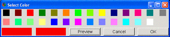
The Color Picker shows a number of colors to select from. There are only a limited number of colors so that the color selection can be easily reproduced on subsequent runs. When you open up the Color Picker, the current (original) color will be in a small box on the bottom left, whereas the box next to it will show the color that was most recently selected. There is a new ``Preview'' button which will change the color and let you see what it would do, but will also allow you to push the ``Cancel'' button and return to the original color, shown in the bottom left.
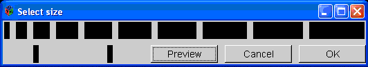
The Size Picker shows 10 sizes to select from, currently (to change later) represented by the size of boxes, where the width of the box represents the selectable size. When you open up the Size Picker, the current (original) size will be represented in a box on the bottom left, whereas the box next to it will show the size that was most recently selected. There is a new ``Preview'' button which will change the size and let you see what it would do, but will also allow you to push the ``Cancel'' button and return to the original size, shown in the bottom left.
Rather than having to open the Size Picker over and over, map3d provides a few options that can be changed by a single keystroke. To do this, open the menu in the Geometry Window and select ``Mesh->Use +/- to select'' and then select a feature you wish to dynamically adjust. Then press + or - to adjust the size. However, most of these only have 10 possible sizes.
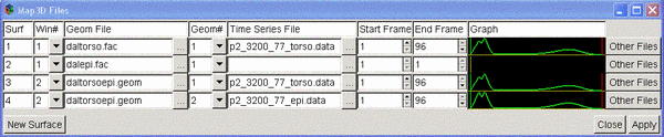
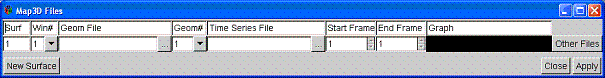
This version of map3d adds new GUI support. The most noticeable new addition is the ``map3d Files'' window, allows you to interactively select filenames, data windows, etc. The others are for saving files, and for quick scaling changes.
The ``map3d Files'' window can be accessed by the ``Files'' menu option of the main menu. This window displays one row for each surface, where each row shows the surface number, the window the surface appears in, the geometry filename, the geometry number, the data filename, the start frame number, the end frame number, a graph of the RMS curve, and a button to show other files. Most of these columns can be modified at any time. If you click on the ``New Surface'' button, an empty row will pop up, allowing you to add a surface from scratch.
None of the changes you make will take effect until you click on the ``Apply'' button. If you click on the ``Close'' button, the window will close, but if you open it again, it will look exactly as when you closed it.
| ||||||||||||||||||||
Also note that this window allows you to run map3d without any arguments. If you do so, or if map3d3d determines that none of the geometry files were valid, the files window will pop up with an empty row waiting for input. If you try to close this window without any input, map3d will treat is as though you were exiting the program.
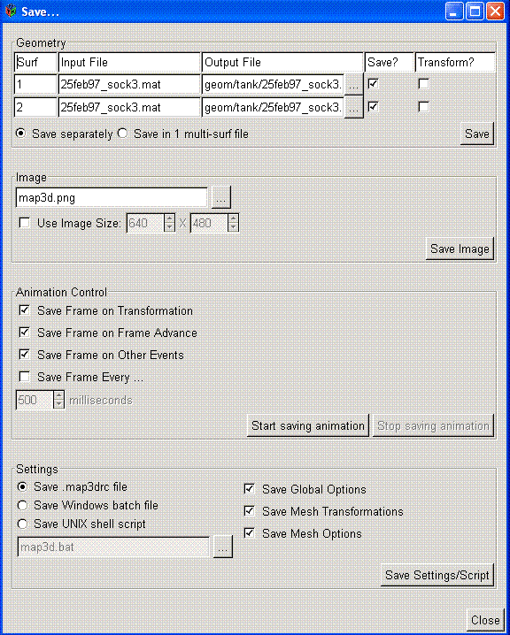
The ``Save...'' Window will display if you select ``Window Attributes->Save...'' from the menu. The first section is to save geometry files, the second is for images, and the third for settings.
In the Geometry section it displays each surface number with its current geometry filename. Next to each there is a check box. If that check box is checked when you click one of the save buttons, then that surface will be one of the ones that is saved. If the second check box (labelled Transform?) is checked, then map3d will save the geometry will be saved with the current transformations (translations and rotations) applied.
Make sure to modify the filename or the current filename will be replaced (if you click on ... you can browse for a filename). If the filename ends in the extension .fac, it will save filename.fac and filename.pts. If the filename ends in .geom, it will save the file in the CVRTI binary file format (see Section 6.1.3). If Transforms is selected and there is a landmarks file, then a filename.lmark.
Clicking on the ``Save in 1 geom file'' button will save all of the geometry into 1 CVRTI binary file (see Section 6.1.3), choosing the filename of the first entry, which must have a .geom extension. Clicking ``Save individually'' will save each in its own filename. There is currently a known bug with saving .geom files under Windows and reading them back in again.
In the image section, select a filename (you can click on ... to browse for a filename) and click save. The filename may have the extension .ppm, ,png, or .jpg to save in one of those formats. The final filename also appends a 4-digit number before the extension, representing a number in a sequence of images. I.e., if the filename selected is map3d.png, the image will actually save in map3d0000.png, and subsequent images will be map3d0001.png, map3d0002.png, etc. The image that will save is approximately the space that all open map3d windows cover.
NOTE: If you have windows that overlap, the one on top might not be the one map3d thinks is on top. So if you move windows around, click inside the window (not the title bar), to tell map3d it is on the top. Otherwise, data you want might be overriden by the data in the window underneath.
If the Save... window is in the way, close it, and pressing the 'w' key will have the same effect as clicking the ``Save Image'' button.
This section allows you to control automatic frame saving to put images together into movies. While map3d is not yet sophisticated enough to actually create the movies, this control can save the images you need and then you can use some external software to make a movie from them. See Section 9.1.2 for links to instructions of how to make movies from sets of images.
There are four controls to select when an image will be saved.
Naturally, animations start recording when you click the ``Start saving animations'' button, and end when you click the ``Stop saving animations'' button. If you close the window while animations are being saved, they will keep recording (this is useful if the Save... window gets in the way of the images you want to save).
map3d saves two types of settings files. There is the .map3drc file, which acts as a settings file which (if in your home directory or in the directory in which you run map3d) will load a list of options at start-time, so map3d can behave similarly each time you run it without having to reset options manually.
The other type of setting file is a script (or batch) file (See Section sec:scripts). map3d will attempt to save exactly what you have loaded, including all files and window positions. The difference between a script and a batch file is that a batch file is designed for MS Windows, and a script is designed for everything else.
To save a script/batch file, click on the appropriate button and select a filename. If you choose to save a .map3drc file, you cannot change the filename.
The only real difference between scripts and the .map3drc file is that the .map3drc file saves global options and the options set on the first surface (which then will apply to all surfaces), and scripts save information about all surfaces. The options they save are the same, so they are grouped together.
These options are added to the command line. For the script, the options are saved as command line arguments, and for the .map3drc file the options are saved to a file and when map3d is executed, the options get inserted into the command line before any other arguments. Note that this also happens when you run map3d from a script. Also note that the options set in the .map3drc file may be overridden by subsequent arguments. (Naturally, both the .map3drc file and the script file may be editted by hand.)
These are three types of options that map3d can save: global options, which are set independent of any surface; surface transformations, which will save the rotation, translation, and scaling of the surfaces; and other surface options, which save everything else. You may select or deselect any of these three items as you wish. Note, if none of them is selected and save a .map3drc file, it will be empty. If none is selected and you save a script, then it will save the filenames and the window information.
The options are as follows (some of these are mentioned in the usage - Section 4). Some of the values are unclear (like the -sc scaling option) as to what the result will be if you edit it by hand. Future versions of map3d will make this more clear. See Section 7 for more information on these features.
| ||||||||||||||||||||||||||||||||||||||||||||||
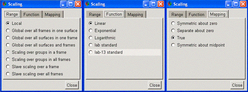
This dialog is pretty much a duplicate of the Scaling Menu in the Geometry menu, but in dialog form for convenience sake. Click on the tab at the top of the scaling type you wish to change (Range, Function, or Mapping), and click on the check box of the feature you wish to select, and map3d will update. (see Section 8.2.3, scaling menu)
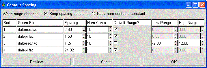
This dialog allows you to select the contour spacing, number of contours and scaling range. A side-effect of this dialog is that if you change one feature, it will change another feature. I.e., if you change the number of contours, then it will also change the spacing.
As a result, there are three buttons on the top of the dialog to select which feature you want to hold constant. So if you select "Keep spacing constant", and change the number of contours, then it will compute a new range based on the new number of contours and spacing; if you select "Keep num contours constant" and change the range, it will compute a new contour spacing.
Note: for the resulting range to be in effect, the ``Scaling range'' (see Sectionsec:scalinggui) must be set to ``user-defined''.
This dialog allows the user to select which Fiducial Contour and/or Fiducial Contour Map he wants to visualize. Under the Fiducial Contour tab the user can select to visualize the Activation Time contour and/or Recovery Time contour or No Fiducials. Under the Fiducial Map tab the user can select to visualize the Activation Time contour map or Recovery Time contour map or No Fiducial maps. The user can also change the contour spacing of the selected contour map.
We are getting many interactive windows in map3d. There are too many to document for each individual feature they control and to show a picture, so instead we will document them in the menu section that opens that particular dialog. Don't worry, if a particular GUI does more than change one or two very simple parameters, we will detail how it works in this section.
By ``picking'' we mean selecting some piece of the display in the current window using the mouse (with buttons). map3d currently supports selection of nodes or triangles with different actions, all of which either return some information, affect the display, or even alter the geometry of the display. In version 5.4, the choices are limited to node information, triangle information, time signal displays, triangulation, triangle deletion, and triangle flipping. Note that picking is successful and the desired results occur only when there is one (no more, no less) hit. To aid in getting the one hit, you may adjust the picking aperture or activate the clipping planes. In any picking mode where your geometry is modified, you might want to save your geometry (see Section 8.5.2). To control picking, use the top-level ``Picking'' menu. See Tables 10 and 11 for the available options.
Pushing CTRL-middle mouse button selects a triangle and kills it, removing it from the list.
There are some lighting and colour controls for the display of landmarks that are useful to know about. Table 21 describes all the specific menus mentioned here.
While screen images are lovely to look at, we need to be able to get the output from the screen to some transportable medium like paper, animation movies, video tape, or film. This section describes some of the methods available for this process.
There are no standard provisions in OpenGL for generating output from the
images generated by map3d. However, map3d uses a collection of the GL
windows to create an image and save it to a file. Once preserved,
this file can be viewed later, either by itself or as part of a sequence of
images in an animation.
To capture an image using map3d simply set the image you want to preserve
and hit the ``w''-key. There will be a slight pause and the a line will
appear in the control window
telling you where the image has been stored. Filenames for image storage
are generated automatically, using the filename specified in the Saving dialog,
which defaults to the value set with the -if option or it will default
to map3d.png (See Section 8.5.2). Appended to this base filename
are sets of four digits, denoting the frame number currently in
the display, starting with ``0001''. Thus, for
example, if the base image file were daltorso.png, the first file
produced would be daltorso0001.png. Note the .png file
extension, standard for this sort of file, can also be changed to .ppm or
.jpg.
The screen area captured in this mode is the smallest rectangle that contains all the windows currently managed by the current invocation of map3d. This often requires with careful placement of the windows or setting the background window for the display to black or something that matches the background of the map3d display.
Sometimes it is desirable to save a sequence of images in a movie for use in a demonstration. map3d does not (currently) have the ability to save movies directly, but it does have the ability to automatically save a sequence of images based on a set of input events, which can be pieced into a movie from external software. The images are saved into a sequence of files based on the rules in the image capture section, and each time the appended digits increment. See Section 8.5.2 for more information on how to control the animations.
There are a few commercial programs we have found useful in generating movies directly:
Otherwise, while we are working on integrating movie support directly into map3d, there are a few packages to create movies from your frames.
We are still learning which combinations of settings work best to capture, edit, and save animations. It depends a lot on the context in which you plan to view/show the results. As we learn more, we will share it with you.
Too many to even begin to contemplate. But if there are any you would like exterminated, please send email to map3d@sci.utah.edu (we accept all foreign currency in large denominations, bicycle parts, assorted outdoor gear, but no credit cards).
Here is a short list of those we know about and are currently addressing:
This document was generated using the LaTeX2HTML translator Version 2002-2-1 (1.70)
Copyright © 1993, 1994, 1995, 1996,
Nikos Drakos,
Computer Based Learning Unit, University of Leeds.
Copyright © 1997, 1998, 1999,
Ross Moore,
Mathematics Department, Macquarie University, Sydney.
The command line arguments were:
latex2html -split 3 -no_white -link 3 -no_navigation -no_math -html_version 3.2,math -show_section_numbers -local_icons manual
The translation was initiated by Rob Macleod on 2005-05-21