Diffusion tensor MRI datasets
This page will attempt to document, collect and/or reference various
diffusion tensor datasets, to facilitate research in diffusion tensor
analysis and visualization.
The datasets here are in NRRD format, which is a
human-readable ASCII header and a raw data file. The advantages of
NRRD over comparable formats include its use in SCIRun and the BioTensor
programs, as well as two powerful command-line tools: unu
and tend, which access functionality in the nrrd and ten libraries of
teem, respectively. Unu does operations on N-dimensional
arrays without any application-specific knowledge of what is in the
array; tend does operations on tensor volumes conforming to
the layout described below. As demonstrated below, piping invocations
of these programs together allows a number of non-trivial operations
to be done quickly, and in a way which facilitates data inspection and
batch pre-processing. Both programs can be invoked with no other
command-line options to get a listing of the available sub-commands
and what they do. Note: unless otherwise noted, the
unu and tend commands demonstrated below should work
with teem version 1.6.0 or later; pre-compiled
binaries are the easiest way to get started.
The values in the dataset are 32-bit floats (C type "float"),
written in raw, big-endian, which opposite of Intel and AMD PCs
(little-endian), but the same as everyone else (Macs, SGI, Sun, etc).
There are seven values per voxel:
- "confidence": this is a mask image, which is 1.0 in regions where
the tensors are meaningful and useful, and 0.0 where the tensors are
noise (such as air). This is not always a sharp threshold: some
fuzziness of intermediate values allows this volume to be isosurfaced
usefully (at value 0.5).
- Dxx
- Dxy
- Dxz
- Dyy
- Dyz
- Dzz
The Dxx, Dxy, ... values are the six unique entries in the (symmetric)
diffusion tensor, as measured in the scanner's coordinate system. If
exact units are known for the tensor coefficients are known, they are
indicated per-dataset.
Communicating sampled tensor fields is complicated by issues of raster
order and coordinate transforms, and these need to be described in
order for the data to be interpreted meaningfully. There are actually
three coordinate systems relevant for describing a sampled tensor
field:
- The measurement frame: the coordinate frame in which the tensor
is represented as a matrix (the Dxx, Dxy, ..., values listed above).
- The sampling frame: The regular grid on which the tensor samples
lie in space. It has three perpendicular axes which span the spatial
domain of the tensor volume.
- The raster frame: Not really a frame on its own, just an ordering
of the axes of the sampling frame, and an ordering of the samples
along the axes of the sampling frame, as imposed by the ordering of the
sample values in memory or on disk.
Starting with the assumption of a right-handed ordered basis {X,Y,Z}
for the measurement space in which the tensors are expressed, we
impose the convention that the sampling frame's axes are also aligned
with the X, Y, and Z directions. This in turn imposes an ordering
and a direction on each of the axes of the sampling space.
Working from the other direction, that of the underlying ordering of
values in memory or on disk, the three coordinates by which the
samples are indexed can be ordered from fast to slow. As one linearly
traverses contiguous values in memory, one of the coordinates will
change fastest, one coordinates changes "medium" fast, and the
remaining coordinate changes slowest. (For example, in normal
interleaved storage of RGB images, the raster axis ordering from fast
to slow is RGB, horizontal, and then vertical.) The fast-to-slow
ordering of the raster coordinates induces a fast-to-slow ordering of
the axes of the sampling frame.
We adopt the convention that the fast-to-slow ordering of sampling
frame axes, and the ordering defined by the {X,Y,Z} ordered basis of
the measurement frame, be the same. Thus the relationship between the
measurement and raster frames is:
- X = fast
- Y = medium
- Z = slow
Furthermore, samples with
a higher memory location should be spatically located at a higher
coordinates in sampling space.
|
|
The dataset consists of these two files:
|
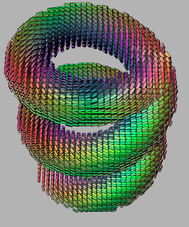
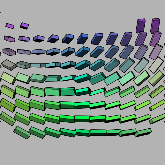
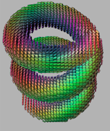
This dataset is a good test or demonstration of the relationships
between the raster, sampling, and world coordinate frames. From fast
to slow, the volume grid dimensions are 38, 39, and 40; errors in this
ordering will result in fragmented structures, looking nothing like
the helical coils shown above in a cuboid glyph rendering. Note that
the coil is right-handed, which determines the correct spatial
ordering of the slices along the Z axis. Finally, notice that the
tensors on the coil surface also twist. If your tensors do not twist
smoothly along the surface of the coil, than the sampling and
measurement frames are in disagreement. Like the helical coils
themselves, this twisting is also right-handed. On the other hand, if
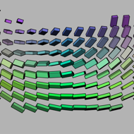
you cut through the diameter of the coils (along the minor eigenvector
of the tensor), and look at how the individual tensors are twisting
(moving vertically in the middle of the second image, aboved), this is
left-handed.
This dataset was created with a tend command from teem version 1.7.0:
tend helix -s 38 39 40 -r 0.5 -R 1.2 -S 2 -o dt-helix.nhdr
The renderings above were also generated with teem (as EPS files):
echo "1   1 1 1   -1 -1 -3" \
 | emap -i - $CAM -o emap.nrrd
tend glyph -i dt-helix.nhdr -emap emap.nrrd -bg 0.7 0.7 0.7 -sat 0.8 \
   $CAM -ur -0.92 0.92 -vr -1.0 1.2 \
   -psc 345 -gsc 0.03 -atr 0.6 -o whole.eps
tend slice -i dt-helix.nhdr -a 2 -p 0 \
 | tend glyph -emap emap.nrrd -bg 0.7 0.7 0.7 -sat 0.8 \
   $CAM -ur -0.3 0.3 -vr 0.2 0.8 \
   -wd 1.6 0.8 0 -psc 900 -gsc 0.03 -atr 0.6 -o slice.eps
rm -f emap.nrrd
Acknowledgment: Something along these lines would be appreciated,
but is not required:
Synthetic tensor dataset produced with the tend program in
the Teem toolkit; <http://teem.sourceforge.net>
|

|
The dataset consists of these two files:
|
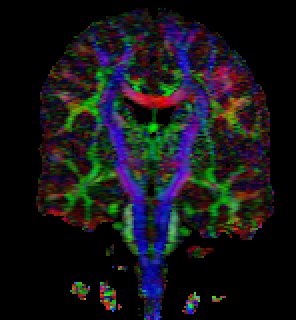
This is a 148 x 190 x 160 scan of Gordon
Kindlmann's brain. The voxel size is
1mm x 1mm x 1mm. MRI Scanning parameters for this
data are not currently available.
Beware that not all samples have positive eigenvalues: probably due to
noise, and the fact that only 6 diffusion-weighted images were used,
so that there was no redundancy in the tensor estimation. Hence, you
may want to run the data through "tend evalclamp"
The first image above was generated by:
tend slice -i gk2-rcc-mask.nhdr -a 1 -p 90 \
 | tend evecrgb -c 0 -a fa \
 | unu axdelete -a -1 \
 | unu resample -s = x2 x2 -k box \
 | unu quantize -b 8 -o gk2-y90.png
The second image, a glyph-based visualization of the same slice, was
created by these steps; the ray-tracing
took a few minutes.
Acknowledgement: If you use this data in publication, you must
provide the following acknowlegement:
Brain dataset courtesy of Gordon Kindlmann at the Scientific Computing
and Imaging Institute, University of Utah, and Andrew Alexander, W. M.
Keck Laboratory for Functional Brain Imaging and Behavior, University
of Wisconsin-Madison.