 |
Carlos Eduardo Scheidegger
cscheid@cs.utah.edu
UID:
00454219
For this final project, I implemented line detection. My implementation is pretty straight-forward. After prefiltering with an appropriate technique, I use the Canny and Marr-Hildreth edge detection to get binary images for the Hough transform. The hard part was to detect the features in the accumulator space. The approach I used was to create a binary version of the Hough transform with the high hits and then cluster that with a hierarchical clustering algorithm. The final clusters are then searched for high accumulation, and these points are transformed back into lines on the image space. In the next sections, I'll describe each of the steps in detail.
I implemented this technique as a sequence of small VISPack programs, so that I could experiment with the individual steps. The source code is provided in the code directory with the submission.
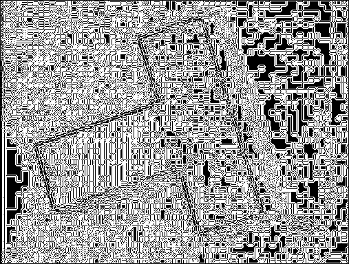
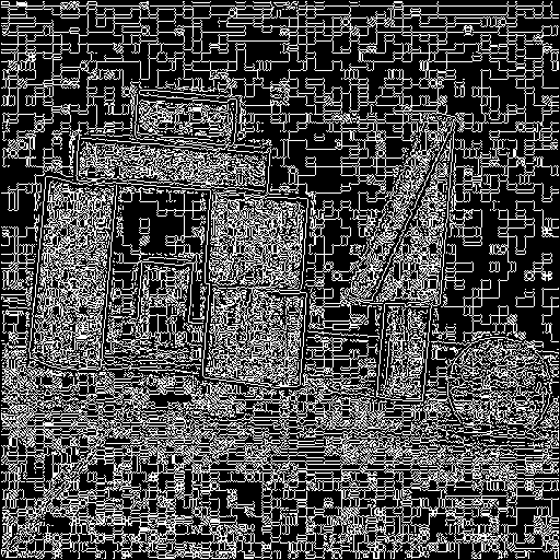
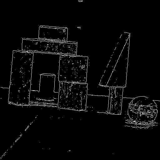
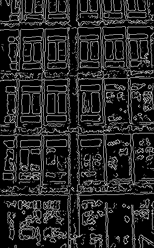
The two edge detection algorithm I used are based on zero-crossings of derivatives. Because of that, they are notoriously sensitive to noise. The usual solution is to prefilter the images or the kernel, whenever the edge-detection kernel is linear.
With appropriate filtering and thresholding, the marr-hildreth does give surprisingly good results. The filtering is essential to get the edges at the correct scale. Unfortunately, it is easy to get parameters wrong:
I then experimented with another filter, the Canny edge filter. The idea of the canny edge filter is to detect maxima of gradient derivatives on the direction of the gradient. Canny also introduced the idea of hysteresis thresholding: using two thresholds and connected components to filter out noise. Since I'm using VISPack's implementation of the Canny edge detection, and it only takes a single threshold value, I imagine that the hysteresis threshold is not implemented.
For the Canny edge detection, I tried using two different forms of filtering: anisotropic diffusion and median filtering. The anisotropic diffusion seemed to work reasonably well, but the edges tended to be ``scruffier'': they are not as neat as the usual detection. I think that may be a bug in my use of VISPack's anisotropic filtering -- I don't think I could get the parameters to work nicely. Here, I'm using between 0.1 and 0.3 and 15 iterations of diffusion. What I found with AD is that I can use much higher thresholds and the results are still adequate.
 |
 |
 |
It seems that median filtering works best for the tests I did. I'm sure that there's something wrong with my anisotropic diffusion, but I couldn't fix it. All in all, Canny edges seemed more robust, especially when there are many edges on the image, because Marr-Hildreth edge detection needs to work on a large scale to get rid of noise issues, and this also suppresses many legimitate edges.
After detecting edges on the images, the main algorithm of the project
is invoked. The Hough transform takes a binary image, and transforms
every lit point in this image to a dual space, usually called the
accumulator space. In this dual space, every point becomes a line (or
a curve). The most important feature of the dual space is that points
that are collinear in the primal space intersect at the same point in
the dual space. Any dual point-line transformation works, but the
normal equation duality is usually employed because of issues like
unbounded values on the parameter space. In this dual transformation,
one dimension (in our case, ![]() )is the signed distance
)is the signed distance ![]() from the line
to the origin. I normalize the image range to
from the line
to the origin. I normalize the image range to ![]() , so
, so
![]() . The other parameter is the normal
of this line, which I call
. The other parameter is the normal
of this line, which I call ![]() . All lines can be represented uniquely
using a range of only
. All lines can be represented uniquely
using a range of only ![]() radians. I normalize the Hough space to
radians. I normalize the Hough space to
![]() by linear scaling.
by linear scaling.
To detect lines, I note that since the image and accumulator spaces are dual, a single point on the accumulator space indicates a line on image space. So I need only pick adequate points on the accumulator space and transform them back. It turns out that this is the hard part.
For images with few edges or little noise, the accumulator space is reasonably well-behaved - the maxima can be picked out somewhat simply looking at local maxima and thresholding. I tried this first approach and it did work on simple images, but it didn't on more complex ones.
My second try was to successively pick global maxima and suppress the
neighborhood (up to a certain percentage of the value on the
accumulator space). This gave better results, but it was hard to tune
the amount of suppression, since it changed a lot from image to
image. My final implementation thresholds the accumulator space in a
different way. I noticed that the points with high accumulation have
markedly high gradients. They are not exactly edges, but edge
detection algorithms should pick those up pretty easily. Then, the
thresholding parameter could be used to filter out false positives. It
turned out that rarely edge detection algorithms detect two closely
parallel lines (unless they're there to begin with). This means that
in the ![]() direction of the accumulation space, the gradient is
usually close to the number of points accumulated in the line. Because
of that, I threshold the Canny edge detection based on the
expectation of the size of the minimum line. I used between 20 and 30
in the examples here.
direction of the accumulation space, the gradient is
usually close to the number of points accumulated in the line. Because
of that, I threshold the Canny edge detection based on the
expectation of the size of the minimum line. I used between 20 and 30
in the examples here.
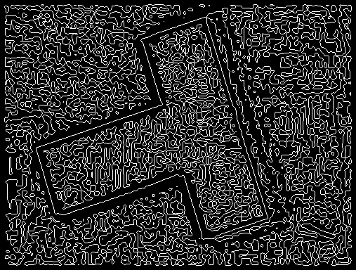
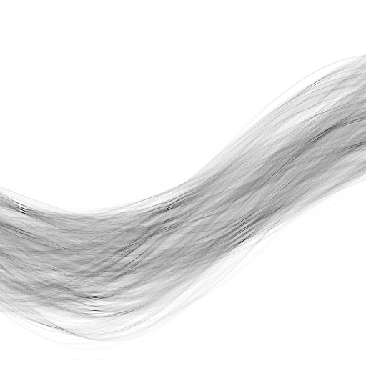
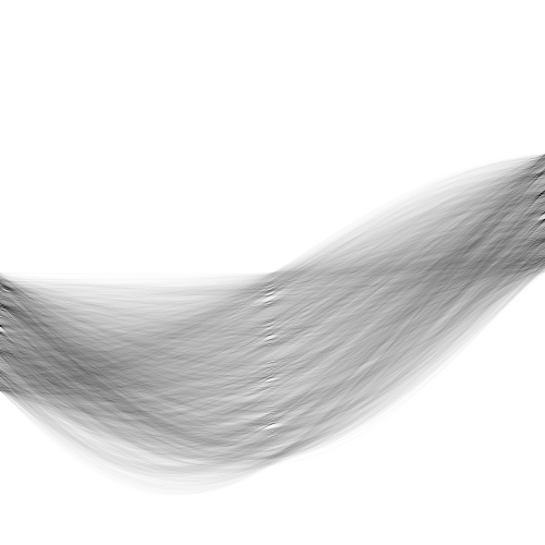
After the edge detection in the Hough space, we end up with another binary image. Each of these points indicate a candidate for transforming back to lines in the image space. We should expect these points to be clustered together, and that is indeed the case:
What is left to do is to cluster these points in coherent bundles, and
use a single line for each of them. I implemented this by simple hierarchical
clustering. Starting with each point representing a cluster, the algorithm try to
find good matches in terms of distance in the parameter space. Instead
of storing the entire complete graph (which could be ![]() memory),
I use a RANSAC-like algorithm where pairs of clusters are picked and
tested. The best pair is then clustered if their similarity if above
a certain threshold. If the pairs fail the similarity test, the
algorithm terminates.
memory),
I use a RANSAC-like algorithm where pairs of clusters are picked and
tested. The best pair is then clustered if their similarity if above
a certain threshold. If the pairs fail the similarity test, the
algorithm terminates.
To implement this, we need a notion of distance in the accumulation
space. I used an ![]() value ranging in
value ranging in ![]() . This has the
advantage of representing every line uniquely, but has a very
interesting consequence. Since the other parameter in the accumulation
space,
. This has the
advantage of representing every line uniquely, but has a very
interesting consequence. Since the other parameter in the accumulation
space, ![]() , gives the signed distance to the origin, two almost
equal lines with opposite facing normals will be far apart from each
other in a naïve distance measurement (the
, gives the signed distance to the origin, two almost
equal lines with opposite facing normals will be far apart from each
other in a naïve distance measurement (the ![]() sign will be
flipped). It turns out that the topology of this parameter space is
exactly the one of the Möbius
strip: after one walk across the
sign will be
flipped). It turns out that the topology of this parameter space is
exactly the one of the Möbius
strip: after one walk across the ![]() parameter range, we end up
with a negative
parameter range, we end up
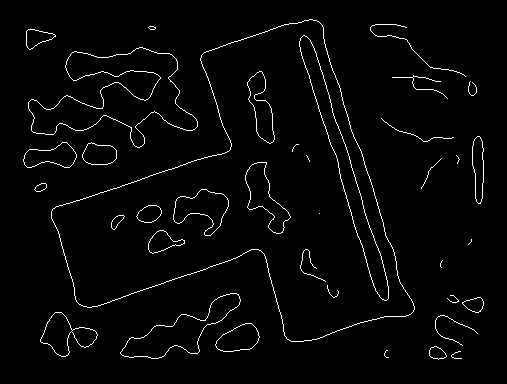
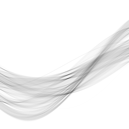
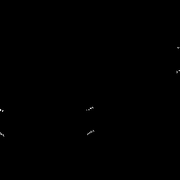
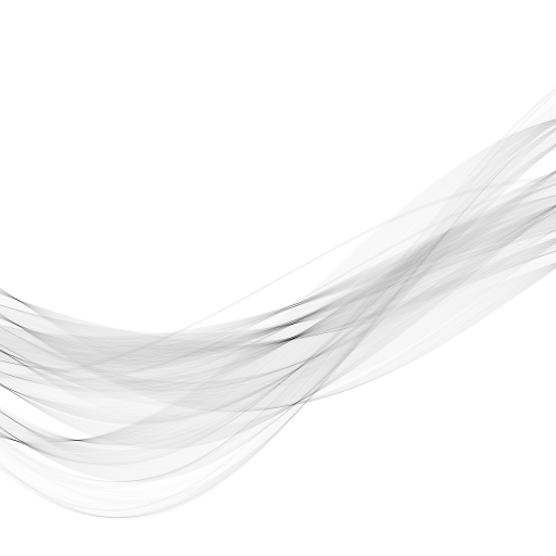
with a negative ![]() . To illustrate this, see this accumulation for
the synthetic square.
. To illustrate this, see this accumulation for
the synthetic square.
 |
The distance measure on the parameter space, then, actually sums
the two ![]() values if
values if
![]() . With such a definition, the
clustering algorithm successfully finds only 4 clusters. Each cluster
is then serached for the highest accumulation. Notice that we have to
search neighboring pixels, because the clusters are actually made of
edges. The transformation back to image space is straightforward.
. With such a definition, the
clustering algorithm successfully finds only 4 clusters. Each cluster
is then serached for the highest accumulation. Notice that we have to
search neighboring pixels, because the clusters are actually made of
edges. The transformation back to image space is straightforward.
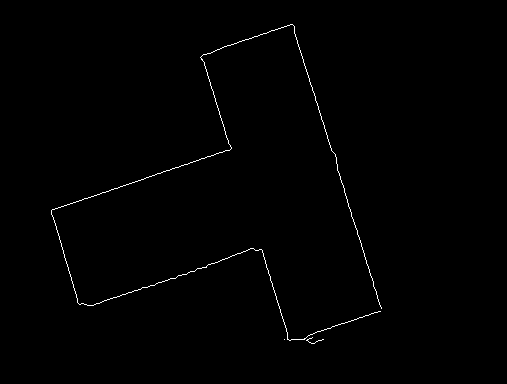
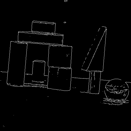
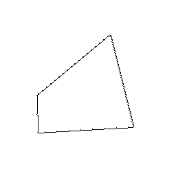
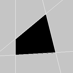
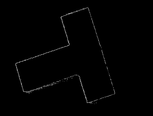
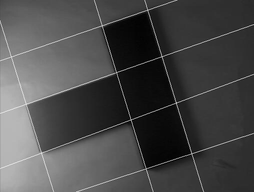
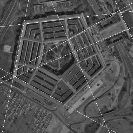
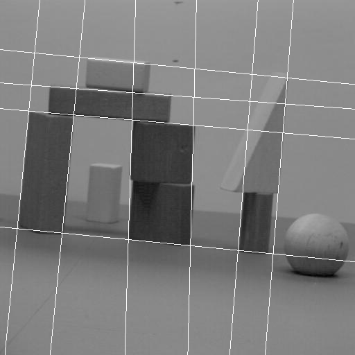
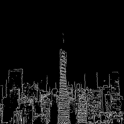
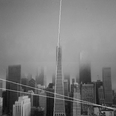
For synthetic data, the Hough transform worked extremely well. Not only few edge outputs from Canny edges make the Hough transform faster, but the absence of noise points cause the accumulation space to be clean, and then the clustering algorithm finds good results. The original image was darkened by 50%, and the detected lines are depicted in white.
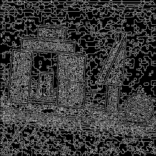
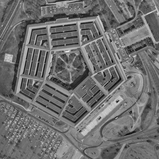
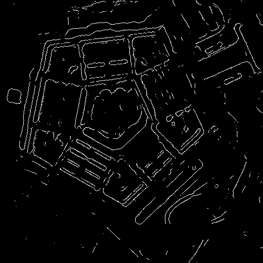
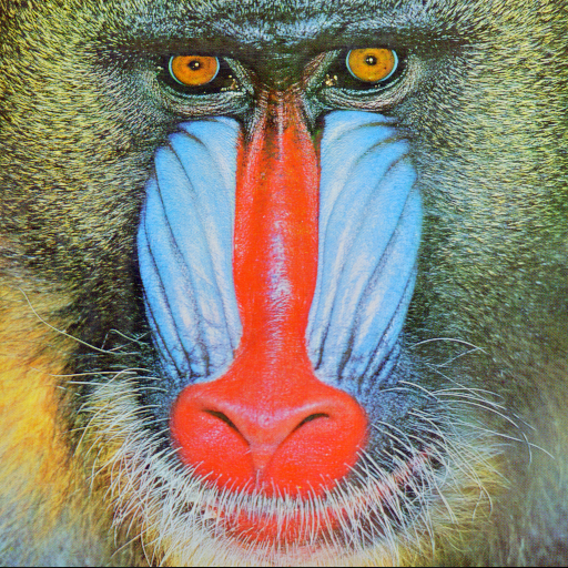
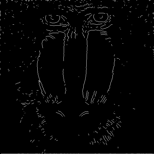
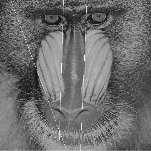
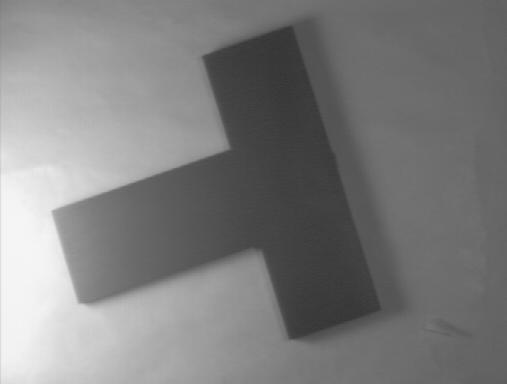
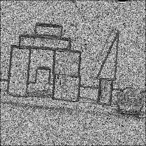
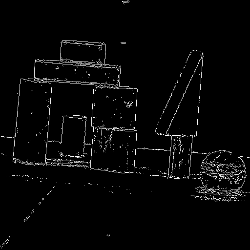
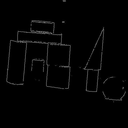
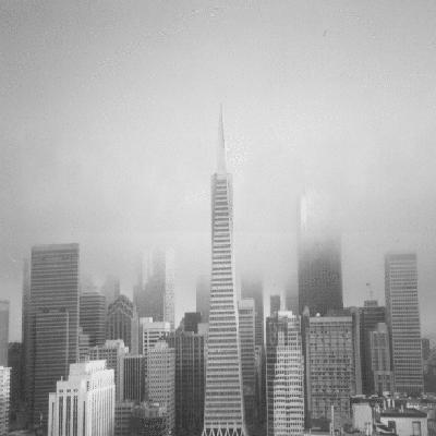
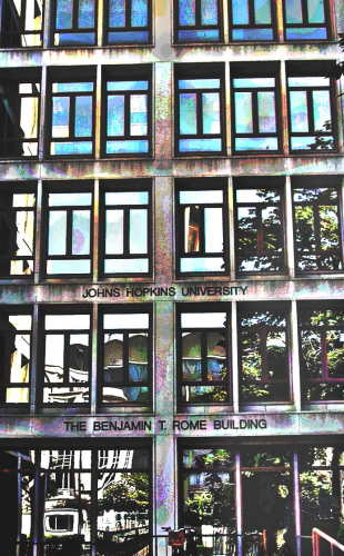
For real photographs, I usually found that median filtering followed by Canny detection with a small threshold or anisotropic diffusion followed by Canny detection with a large threshold gave best results. There was only one instance in which the Marr-Hildreth performed best, and that was with the Baboon image, where the Marr-Hildreth detection succesfully found the two main lines of the baboon's nose. Still, it required significant parameter tuning.
 |
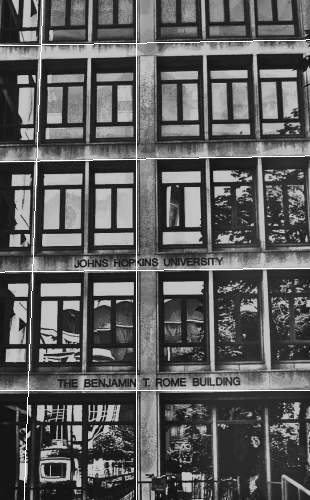 |
Most of the results are reasonable. There were some inexistent lines, like for example the diagonal lines on the buildings example, and the horizontal line in the bottom of the baboon. Still, I believe that my implementation got good results on a variety of images.
I also think my edge detection on the Hough transform is not that good. I can definitely pick out the maxima by eye, so I believe there has to be a way of doing it automatically. I'm pretty happy with the clustering algorithm, but if it gets wrong input data, it will output bad data (such as can be seen in the buildings example).
Overall, I had a lot of fun coding these projects up throughout the semester, and it did give me a much deeper understanding of the subject than I would have had otherwise. It was a lot of work, but it was definitely worth it.
This document was generated using the LaTeX2HTML translator Version 2002 (1.62)
Copyright © 1993, 1994, 1995, 1996,
Nikos Drakos,
Computer Based Learning Unit, University of Leeds.
Copyright © 1997, 1998, 1999,
Ross Moore,
Mathematics Department, Macquarie University, Sydney.
The command line arguments were:
latex2html -split 0 -nonavigation index
The translation was initiated by Carlos Scheidegger on 2005-05-06