 |
(1) | ||
| (2) | |||
 |
(3) | ||
| (4) |
Carlos Eduardo Scheidegger
cscheid@cs.utah.edu
UID:
00454219
|
(1) | ||
| (2) | |||
|
(3) | ||
| (4) |
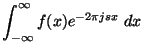
and the power spectrum by
| (5) | |||
| (6) | |||
| (7) |
We will use the power spectrum to visualize the frequency domain of
both images and filters. In typical scenarios, the power spectrum has
much higher dynamic range than their spatial domain
transforms. We don't usually care about the specific values in
each point for visualization purposes. So we will use the logarithm of
the power spectrum to compress the dynamic range. Since most typical
images tend to concentrate most of the energy in low frequencies, we
have many values in the frequency domain practically zero. Since
![]() , the logarithm might not compress
the dynamic range as we intended to. To compensate for this, we add a
constant value of 1 to the power spectrum, because
, the logarithm might not compress
the dynamic range as we intended to. To compensate for this, we add a
constant value of 1 to the power spectrum, because
![]() , but
, but
![]() . In
this way, the smallest value is the visualization is zero, and the
large values are mostly unaffected.
. In
this way, the smallest value is the visualization is zero, and the
large values are mostly unaffected.
Computers are eminently discrete computing devices, and so sampling a continuous function is an inevitable step in any digital signal processing application. WE wish to study the effects of sampling in signals.
We model sampling as a multiplication of the original sequence by an infinite sequence of impulses. The relative strength of each impulse will represent the original value of the function at that point. This pulse sequence is known as the Shah functional:
 |
(8) |
The Shah function has several interesting properties. First of all, its Fourier Transform is itself, and it has a nice similarity transformation:
| (9) | |||
| (10) |
(These equations can be proven by taking the limit of a sequence of progressively more compact gaussians [2]) Equation 10 will be particularly useful to understand the consequences of sampling.
This model allows us to accurately talk about the impacts of sampling in the original image. In the discussion, we will use the frequency domain extensively. Specifically, we will investigate what happens to the power spectrum of the original function under sampling. The power spectrum measures the relative strength of the signal for a given frequency.
I implemented three different low-pass filters to reduce the effects of aliasing. All three of them are radially symmetric, to ensure that the entire operation was radially invariant (I wanted to suppress frequencies in the same way across all directions). One of the filters is separable (the Gaussian), while the two others aren't (Butterworth and ideal). I'll explain and analyze each in a separate section.
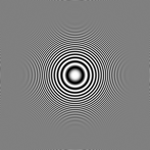
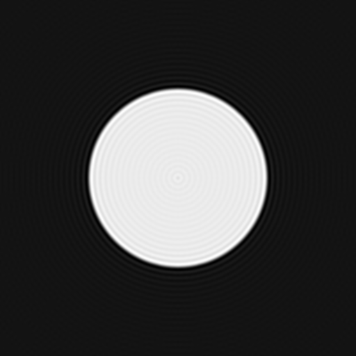
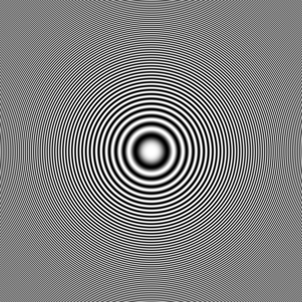
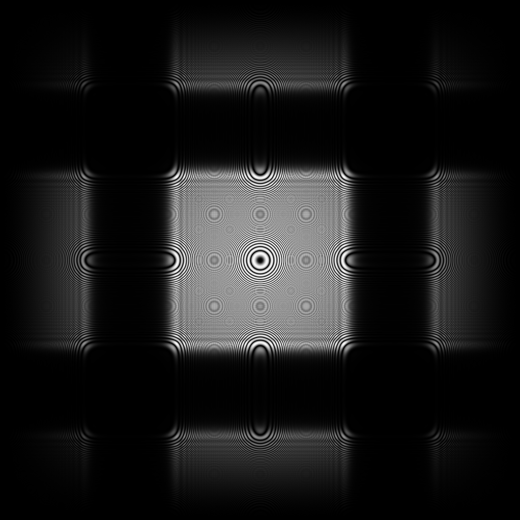
My experiments included synthetic images. To investigate ringing, I tested the filters on images with large discontinuities in color. For that, I used an image with a white square on a black background.
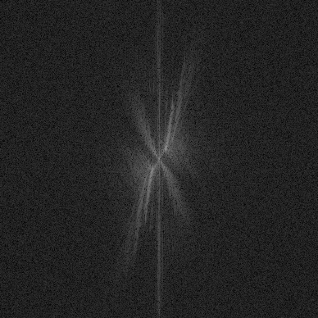
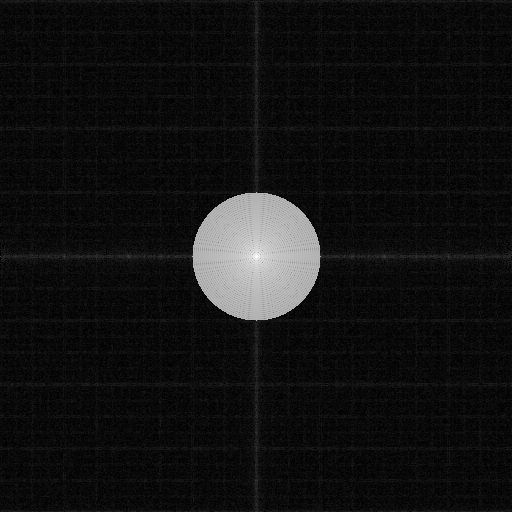
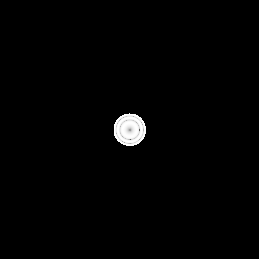
Since the circle is nothing but a radially symmetric rectangle function, its power spectrum is clearly a radially symmetric sinc function. Because the circle is fairly low-frequency, the sinc function is comparably high-frequency. The ringing in Figure 2 is more evident than would be expected because we're visualizing in log space.
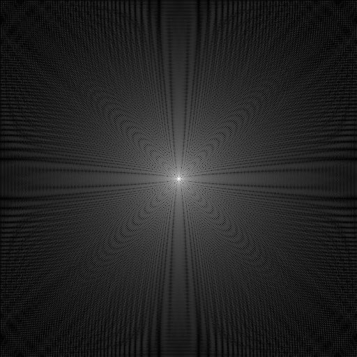
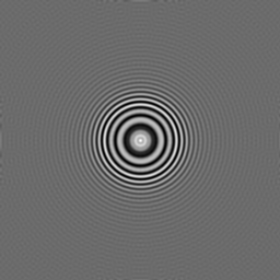
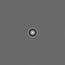
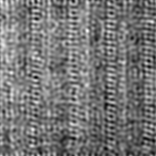
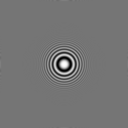
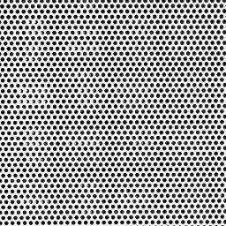
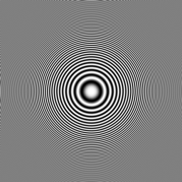
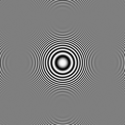
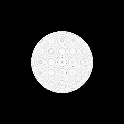
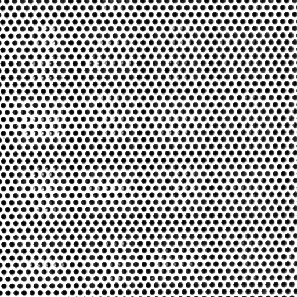
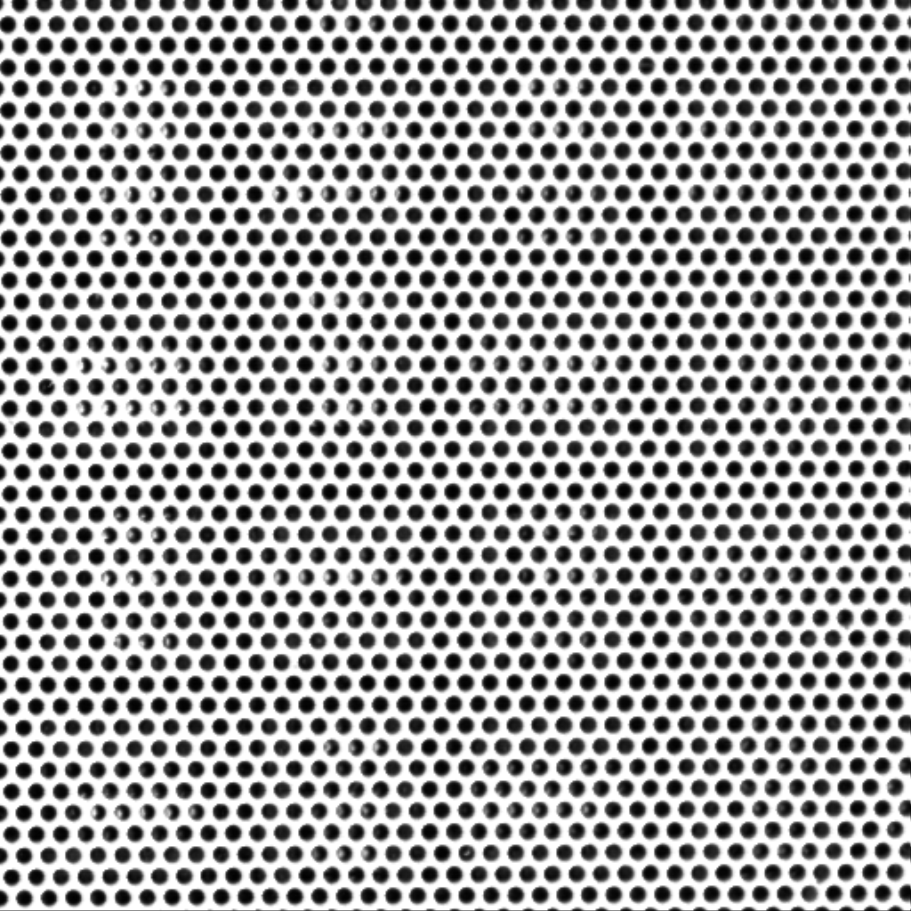
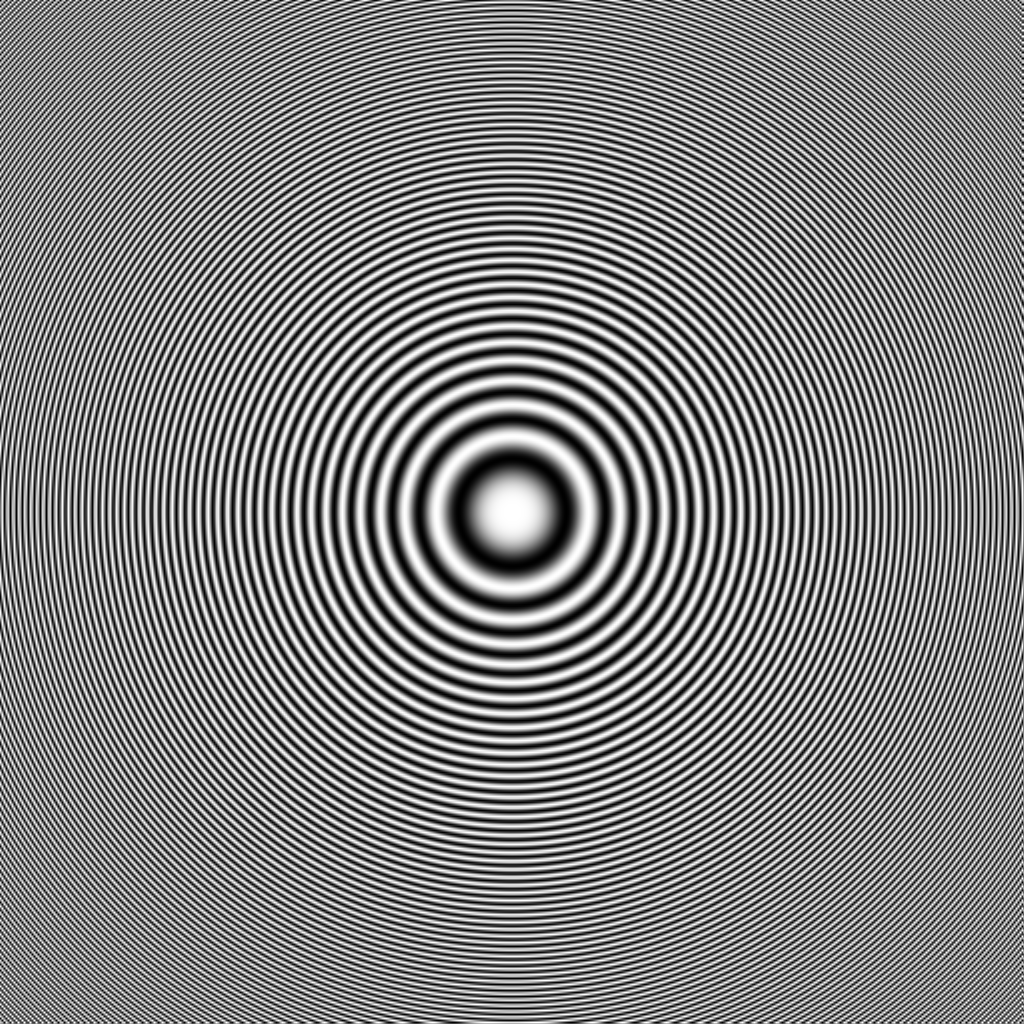
To investigate in-spectrum loss and foldback, I used a
synthetic image with artificially high frequency content. Since I
wanted a radially symmetric image, I decided to use
![]() (later I found out a reference in the web for this function
under the name ``zone-plate'').
This function is interesting. First, its frequencies are increasing
linearly as a function of distance from the origin. This allows us to
deterministically compute the highest frequencies present in the
image. Second, it is almost its own
fourier transform (I used Mathematica for this, but I suspect it can
be done by some form of series expansion):
(later I found out a reference in the web for this function
under the name ``zone-plate'').
This function is interesting. First, its frequencies are increasing
linearly as a function of distance from the origin. This allows us to
deterministically compute the highest frequencies present in the
image. Second, it is almost its own
fourier transform (I used Mathematica for this, but I suspect it can
be done by some form of series expansion):
 |
(11) |
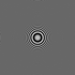
Since the original (before the sampling) images are not really
continuous, we have to be careful not to have any sampling artifacts
in them. I wanted to have as high frequency components as possible in
the original images, so I scaled the radius appropriately. Here, I use
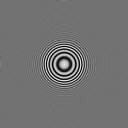
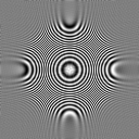
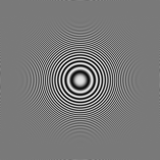
both 512x512 and 1024x1024 zone plates. The sampling theorem states
that the highest possible sampled frequency is half the sampling
rate. Since we're sampling at integral numbers of ![]() and
and ![]() , the
highest frequency we can sample is 1/2. This implies a scaling factor
of
, the
highest frequency we can sample is 1/2. This implies a scaling factor
of
![]() and
and
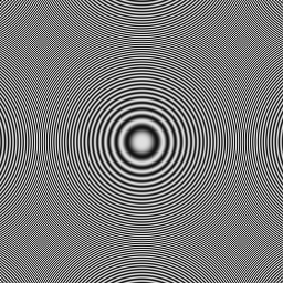
![]() . With this scaling
factor, the frequency of the sampled function will be exactly the
maximum sampling frequency at the corners of the image. There will be
(in theory) no aliasing. The power spectrum will be very similar, but
scaled, because we're scaling the definition to get the desired
frequencies. In practice, we can see some very mild aliasing. I
believe this to be an issue of displays rather than anything else:
I've experienced worse aliasing in CRTs than in LCDs, and the aliasing
becomes really noticeable if you drag the window around (try it, it's
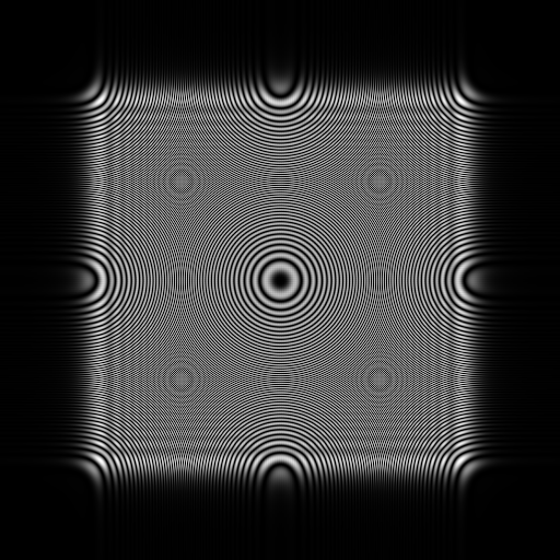
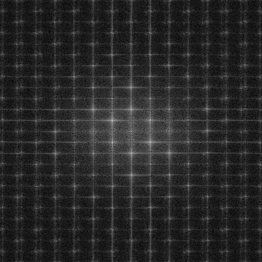
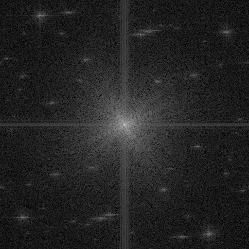
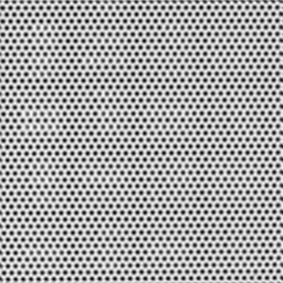
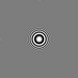
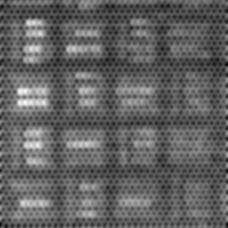
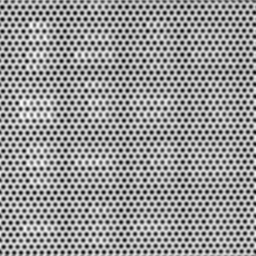
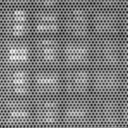
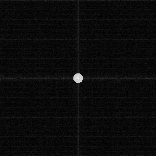
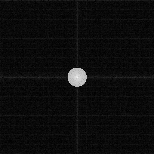
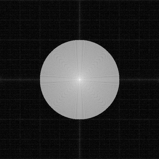
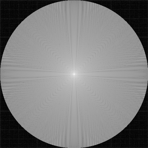
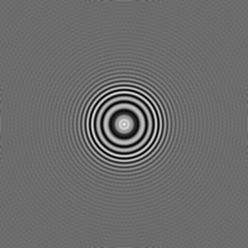
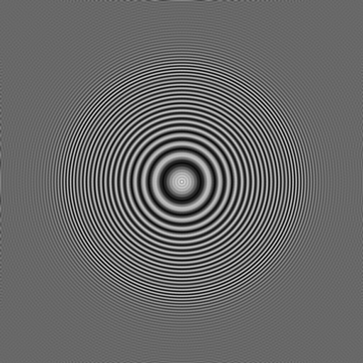
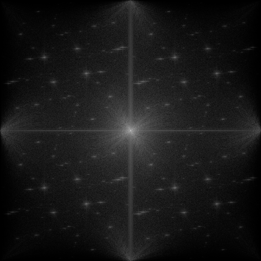
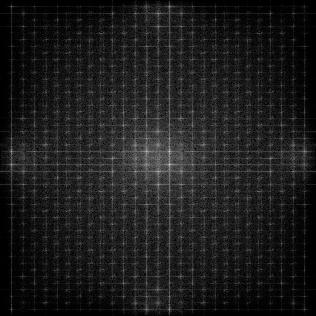
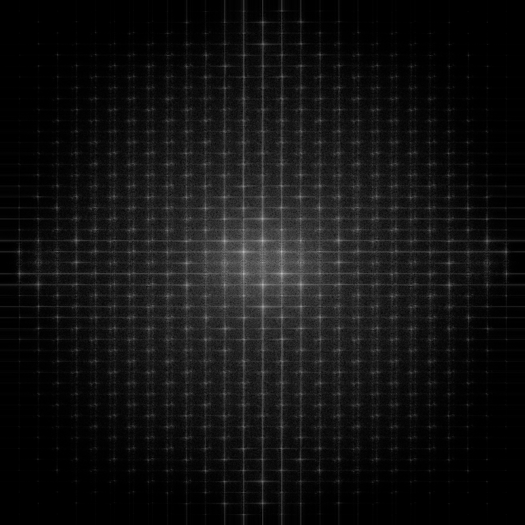
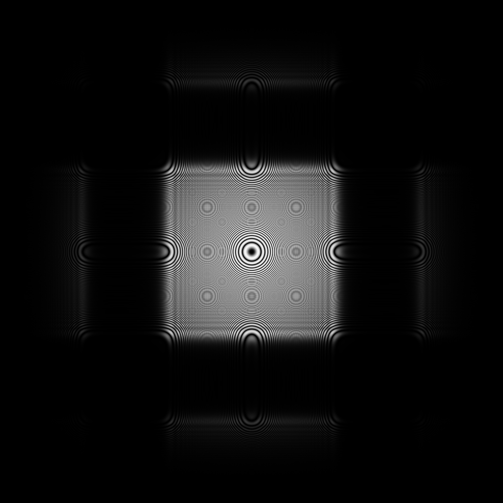
kind of cool). The 512x512 zone plate and its power spectrum are shown
in Figures 3 and 4. The
power spectrum is aliased because of the scaling.
. With this scaling
factor, the frequency of the sampled function will be exactly the
maximum sampling frequency at the corners of the image. There will be
(in theory) no aliasing. The power spectrum will be very similar, but
scaled, because we're scaling the definition to get the desired
frequencies. In practice, we can see some very mild aliasing. I
believe this to be an issue of displays rather than anything else:
I've experienced worse aliasing in CRTs than in LCDs, and the aliasing
becomes really noticeable if you drag the window around (try it, it's
kind of cool). The 512x512 zone plate and its power spectrum are shown
in Figures 3 and 4. The
power spectrum is aliased because of the scaling.
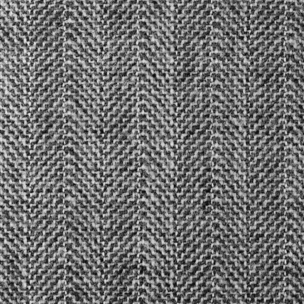
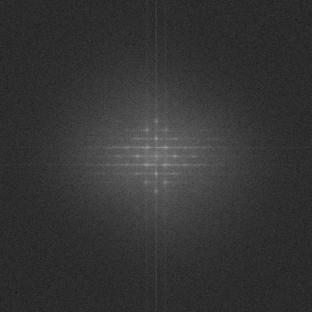
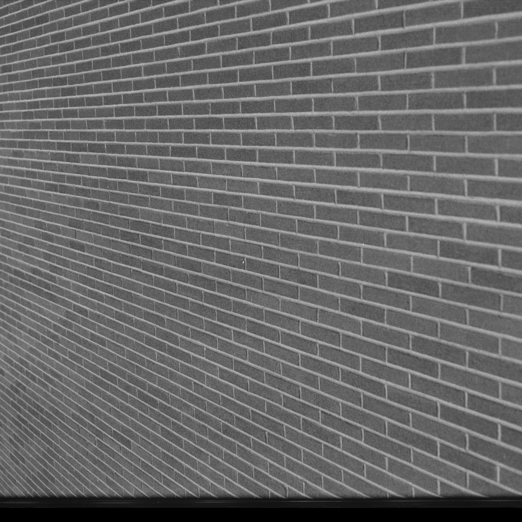
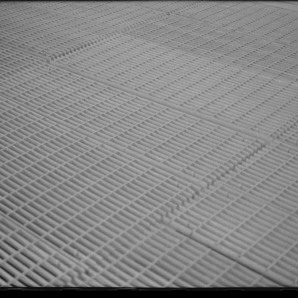
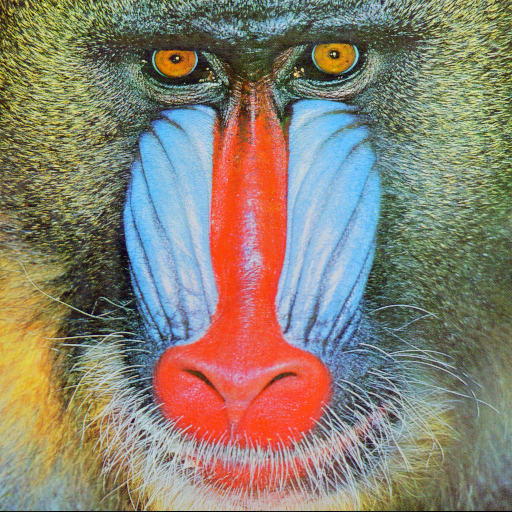
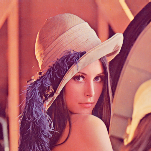
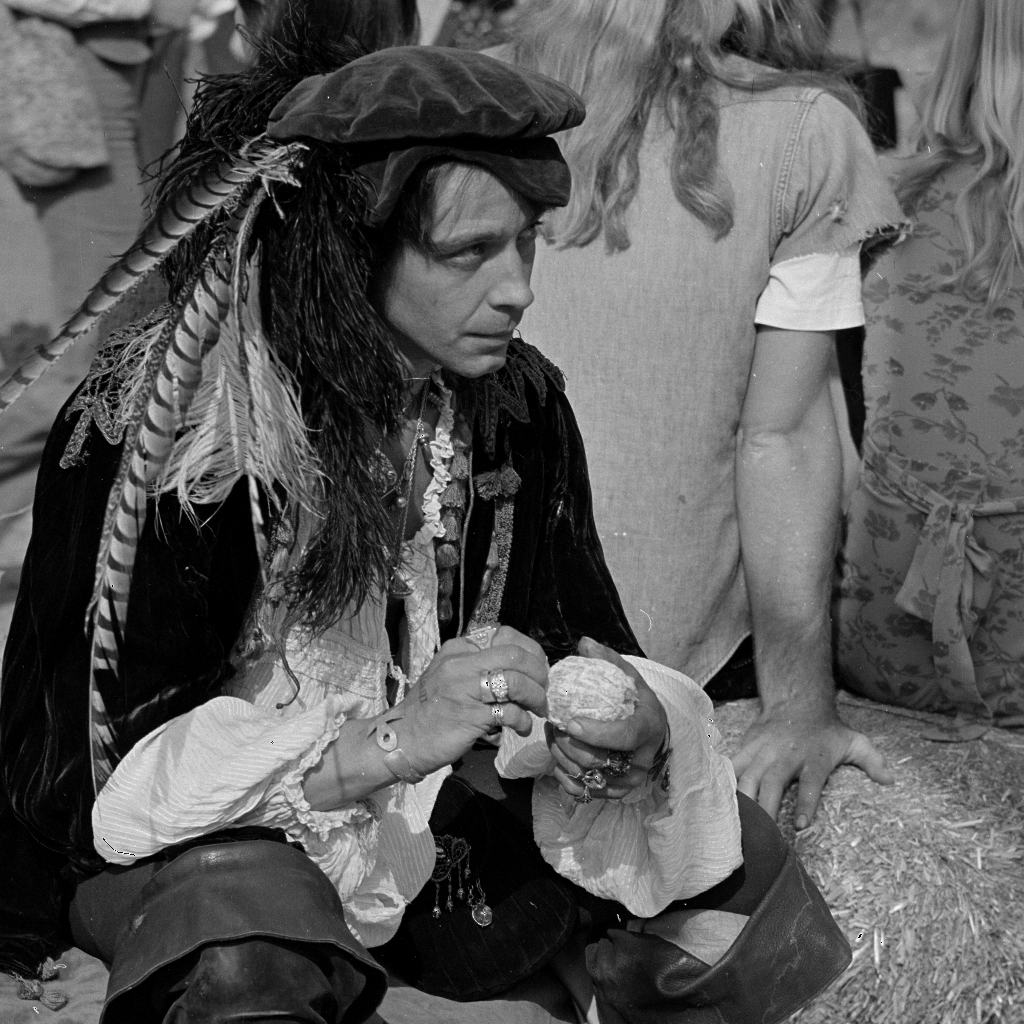
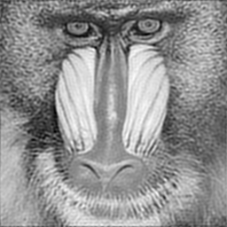
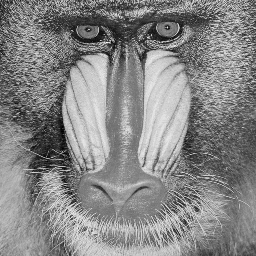
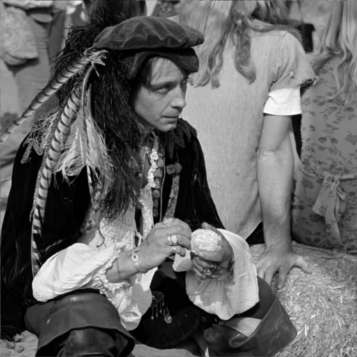
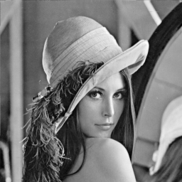
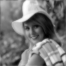
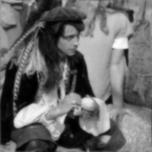
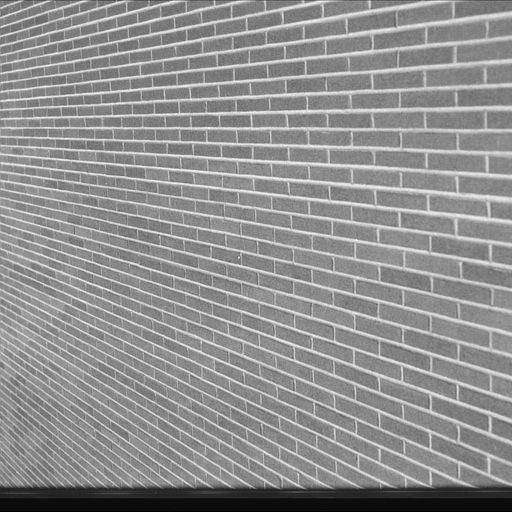
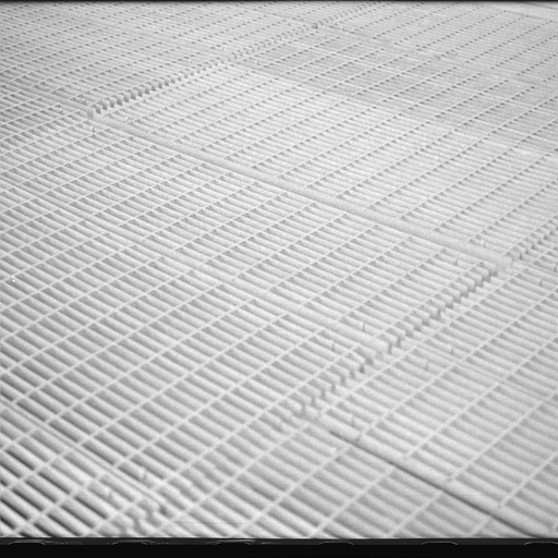
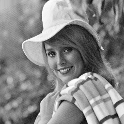
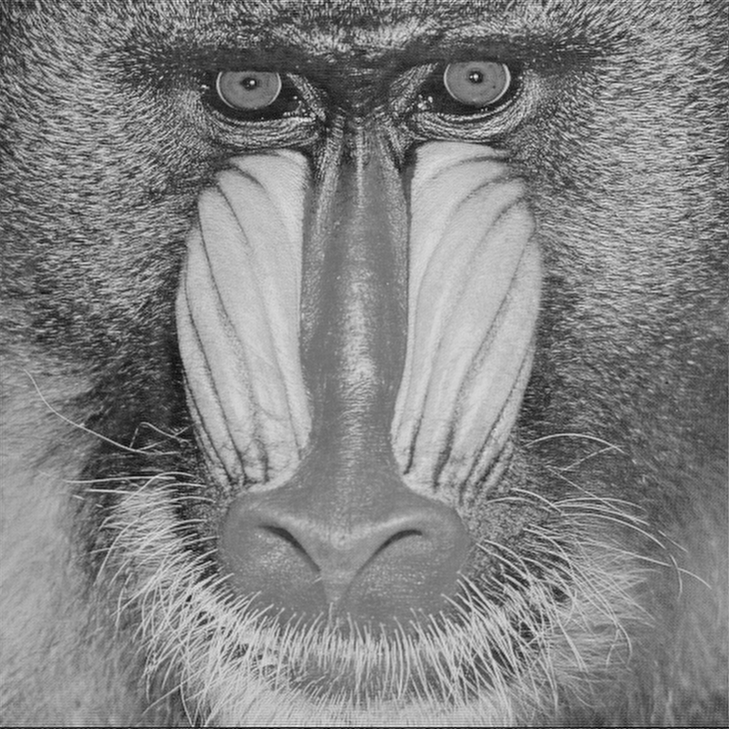
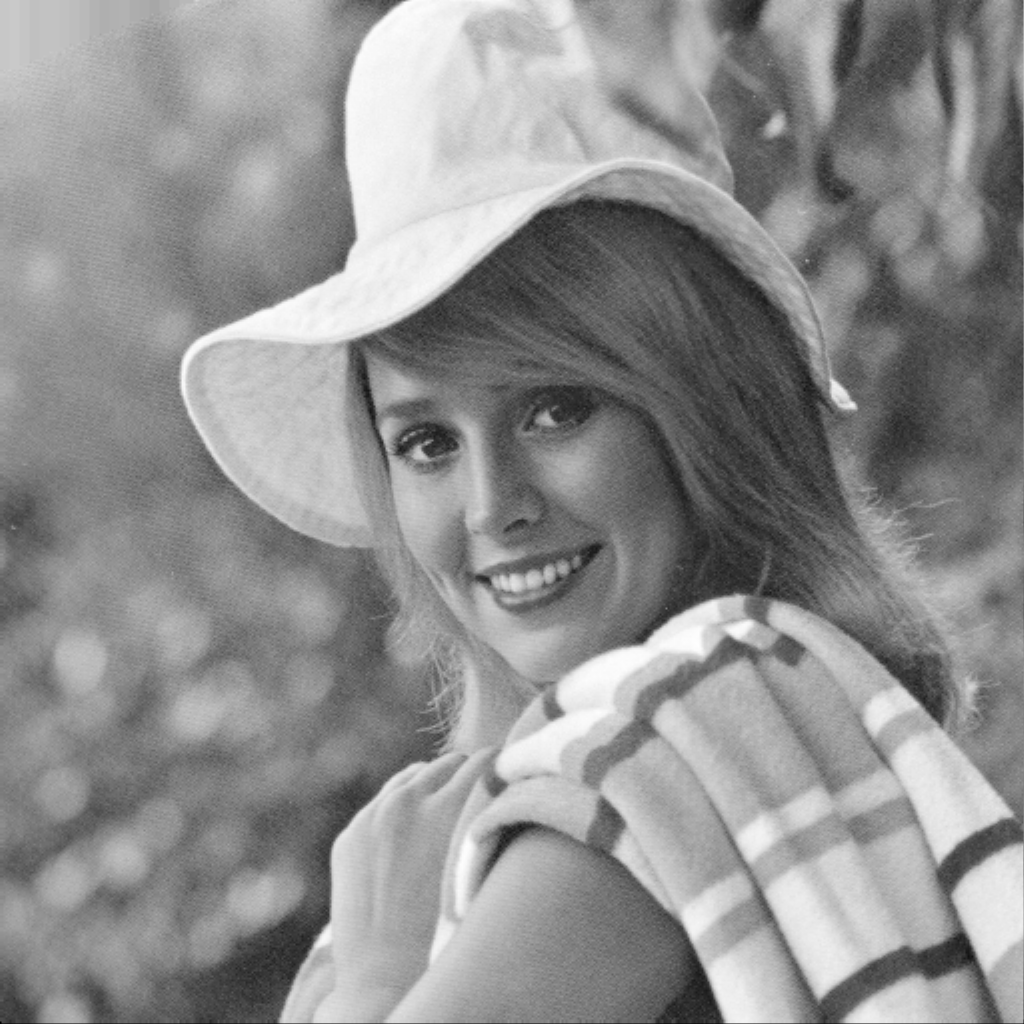
My real-life images were taken from the USC-SIPI database [1]. I chose to use these images because they were specifically collected for the purpose of testing algorithms, and their examples span a big range of image ``features'', such as color, texture, contrast, etc. I tested my filters on images 1.3.05 5, 1.4.01 6, 1.4.07 7, 1.5.02 8, 4.2.03 (the ``baboon'') 9, 4.2.04 (``Lenna'' -- with two `n's [3]), 5.3.01 11 and elaine.512 12. I chose these figure subjectively to span a variety of features such as noise (both white and frequency-specific), resolution, texture, perspective and contrast. I will not refer to all the results in the main text, but I include them as an appendix.
The main sampling artifact is known as aliasing. Since we're modeling sampling as multiplication by a sequence of pulses, the effects of aliasing in the frequency domain are a sequence of convolutions of the image frequencies, displaced by an amount dependendent on the sampling rate: the higher the sampling rate is, the farther apart the pulses are in the frequency domain.
Aliasing is so called because since if the signal we're sampling has energy in frequencies higher than half the spacing between the pulses, the convolution will cause these to overlap. So when we examine the frequency domain of the original function after sampling, some of its higher frequencies will have been ``disguised'' as lower frequencies: they will fold back to the low-frequency spectrum.
To prevent aliasing, we have to make sure that the signal is band-limited before we do the sampling. We then use appropriate low-pass filters for that. In theory, the best possible filter is the one where all frequencies above the sampling rate are suppressed. It turns out this strategy exhibits severe visual artifacts such as ringing, due to what is called Gibbs phenomenon [2]. The solution for that is to use filters with a higher degree of continuity. The consequence is called in-spectrum energy loss: we will reduce the energy of frequencies allowed by the sampling rate we use so that there will be less visual artifacts.
The final effect of aliasing is known as truncation, and happens when filtering a continuous signal with a non-band-limited filter (such as the sinc filter). Since we can only physically construct band-limited signals, I modeled these by multiplying the original filter with a rectangular box function the width of the filter being used. The truncation artifacts then show up as a distortion of the filter in the spatial domain. This distortion is given by a convolution of a sinc function with the original filter. We can then expect some (possibly mild) ringing.
I used 2x and 4x subsampling here. For the case of 2x subsampling, the resulting spectrum is half the size in each dimension. All energies above that will show up as aliasing. We then integrate the filter energies on these regions to give a bound of the expected aliasing. The in-spectrum loss is modeled by subtracting the integral of the in-spectrum filter energy from 1. I model the truncation error as the difference in total energy between the truncated filter and the original one.
The first filter I implemented was the ILPF. The ideal low-pass filter
has a single parameter ![]() that indicates the highest frequency that is to
be present in the filtered images. Frequencies higher than
that indicates the highest frequency that is to
be present in the filtered images. Frequencies higher than ![]() are eliminated entirely from the filtered image, while all other
frequencies are untouched. The following functions describe the filter
in the spatial and frequency domains:
are eliminated entirely from the filtered image, while all other
frequencies are untouched. The following functions describe the filter
in the spatial and frequency domains:
| (12) | |||
| (13) |
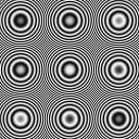
I tested this filter with cutoff frequencies of one-half, 1/4th, 1/8th, 1/16th, 1/32th and 1/64th of the domain width. These should result in progressively increased blurring. Also, since this filter is equivalent to convolving with a sinc function, we should expect noticeable ringing in the filtering. The following figures show the effects of filtering on the synthetic circle and 512x512 zone plate:


 |


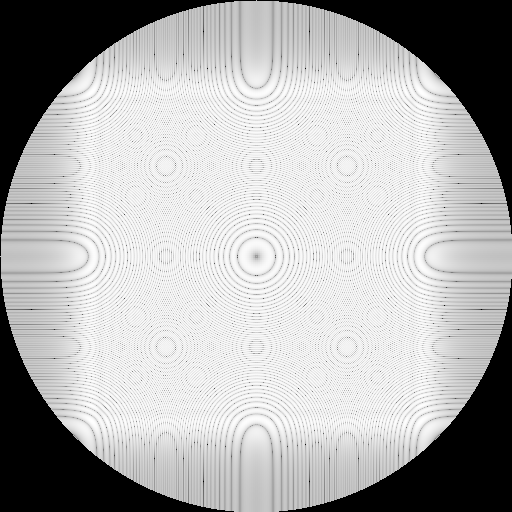 |
The power spectrum became hard to visualize because the filter simply cut off all the frequencies above the threshold, and so the log scale brought up whatever tiny energies there were present. There are some leftover frequencies in the synthetic circle images. Since I first filtered the image and then recomputed its power spectrum, something in that process may have introduced these lower energies. The circle exhibits, expectedly, a very large amount of ringing. The only reason we cannot notice more ringing in the zone plate is that the original image already rings a lot. Surprisingly, the images are not radially symmetric. I think this can be attributed to the truncation in the edge of the filters, or maybe my circles and zone-plates are not perfectly centered.
The subsampled images are shown here.
| ||||||||||||||||||||||||||||||||||||||||||||||||||||||||||||||||||||||||||||||||||||||||||||||||||||||||||||||||||||||||||||||||||||
Here are some figures to illustrate the results. I'll repeat the same idea in the following sections. I chose some overly-blurred images, some good results and some aliased ones. These are already the 2x subsampled images.
It is important to notice that although the some of the images portrayed above exhibit little to no in-spectrum loss and foldback, they still show severe ringing artifacts due to the discontinuity of the filter in the frequency domain (specially the circle, where there's a specific discontinuity). The ILPF performs well on numbers, but the filtering results may not be satisfactory.
| (14) |
For example, it is its own Fourier Transform (up to
scaling). This makes analysis much simpler. Also, since it is
![]() , there will be no Gibbs phenomenon associated with the
filtered images back on the time domain (ie. there will be no
ringing). Finally, Gaussian filters provide a single parameter
, there will be no Gibbs phenomenon associated with the
filtered images back on the time domain (ie. there will be no
ringing). Finally, Gaussian filters provide a single parameter ![]() to adjust, which can be important if there is user involvement in the
process. The main drawback of the Gaussian filter family is that there
can be significant in-spectrum loss, resulting in blurring in the
subsampled images. In practice, I
only experienced this problem in the pathological zone-plate example.
Usually, the Gaussian filter is implemented as a separable filter. I
have not done so here because of simplicity.
to adjust, which can be important if there is user involvement in the
process. The main drawback of the Gaussian filter family is that there
can be significant in-spectrum loss, resulting in blurring in the
subsampled images. In practice, I
only experienced this problem in the pathological zone-plate example.
Usually, the Gaussian filter is implemented as a separable filter. I
have not done so here because of simplicity.
| ||||||||||||||||||||||||||||||||||||||||||||||||||||||||||||||||||||||||||||||||||||||||||||||||||||||||||||||||||||||||||||||||||||
Again, the zone plate was the one function that gave the filters troubles, giving either significant in-spectrum loss or severe leaking. We can definitely see the aliasing effects on the forth and fifth images of the above figure, while the fourth still has 20% in-spectrum loss. The other images, in general, did not exhibit severe problems.
While the gaussian filter can overblur some images, most images that are not overblurred do not exhibit serious aliasing effects. The only image that was not properly filtered was, again, the zone plate. The interesting effect observed in the first overblurred image is due to the peculiar power spectrum of that image 8.
So far, we've seen that the ideal low-pass filter provides good
results in terms of foldback and inspectrum loss, but gives bad
ringing artifacts. The gaussian filter family exhibits no ringing, but
has noticeable inspectrum loss problems. To try and alleviate this,
the butterworth filter family has an additional parameter called the
order of the filter, that provides a way to tune between smooth
and sharp frequency cutoff transitions. The frequency response of the
![]() th-order Butterworth filter I implemented is as follows:
th-order Butterworth filter I implemented is as follows:
 |
(15) |
The ![]() indicates the radius of the frequency response in which the
filter should dampen the energies by 50%.
indicates the radius of the frequency response in which the
filter should dampen the energies by 50%.
The following table summarizes the results for several different
orders (1, 4, 16) of the butterworth filter:
| ||||||||||||||||||||||||||||||||||||||||||||||||||||||||||||||||||||||||||||||||||||||||||||||||||||||||||||||||||||||||||||||||||||
| ||||||||||||||||||||||||||||||||||||||||||||||||||||||||||||||||||||||||||||||||||||||||||||||||||||||||||||||||||||||||||||||||||||
| ||||||||||||||||||||||||||||||||||||||||||||||||||||||||||||||||||||||||||||||||||||||||||||||||||||||||||||||||||||||||||||||||||||
The 1st-order butterworth filter seems too smooth, exhibiting significant in-spectrum loss even for real images, which wasn't the case for the gaussian or ideal filters. It also exhibits foldback, although it's not noticeable from the images. The 4th order butterworth filters seemed to perform adequately, without significant in-spectrum loss or foldback for wider kernels. The 16th order, on the other hand, did suppress foldback entirely for most cases. On the other hand, the 16th order filter is more ``discontinuous'' than the other ones, so the images exhibit more ringing.
Notice that even the zoneplate image exhibits little aliasing. The butterworth filter seems more tunable than the other ones, but in general the gaussian filter is more than adequate and much simpler to tune.
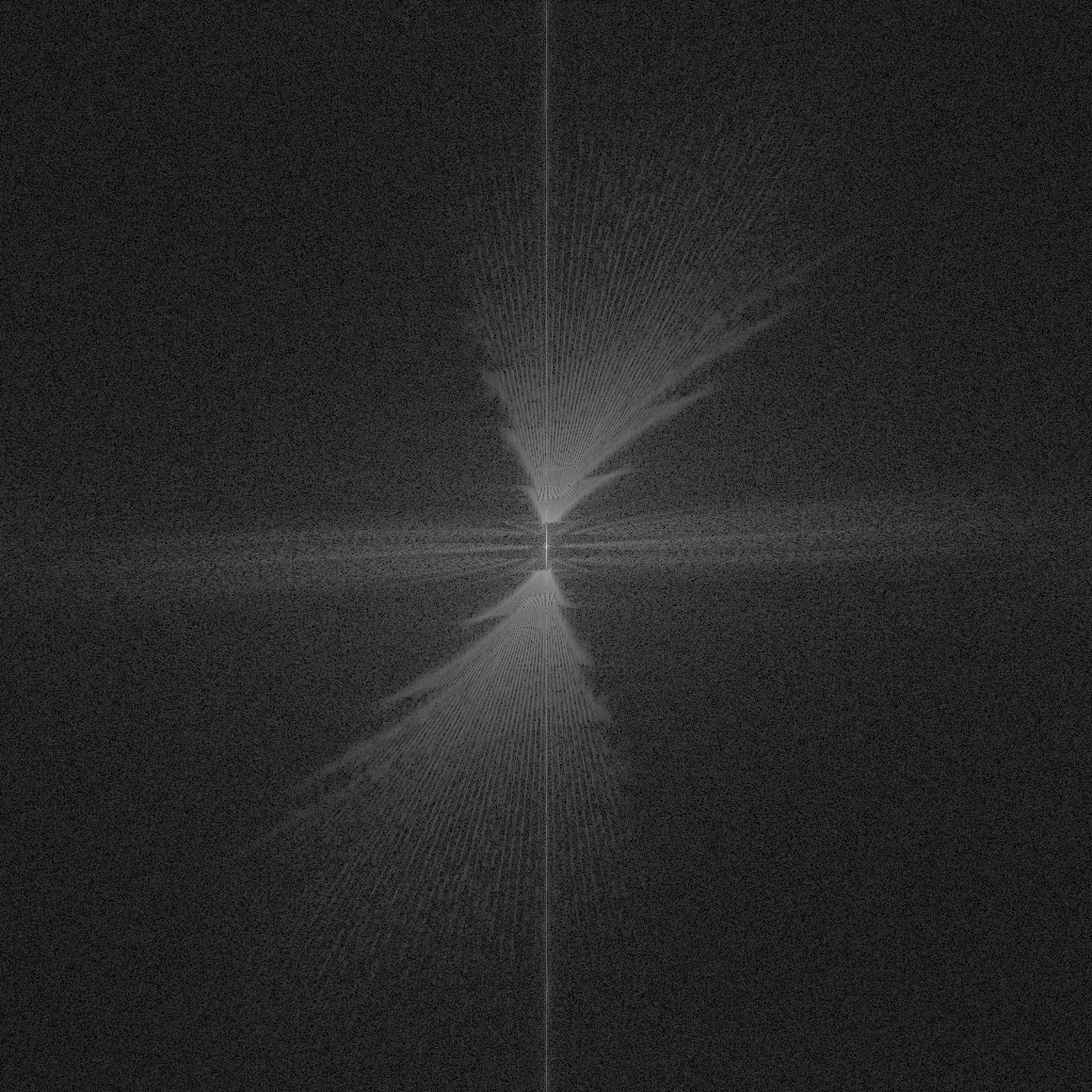
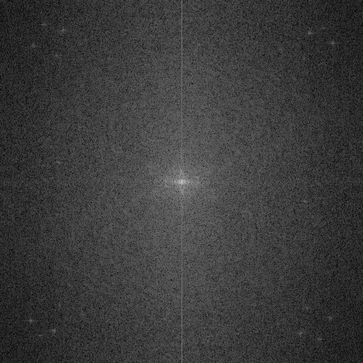
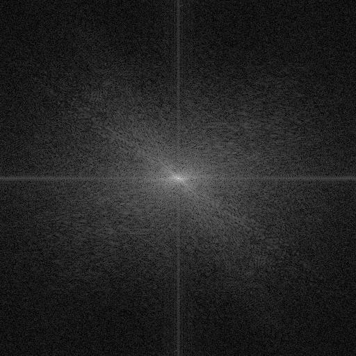
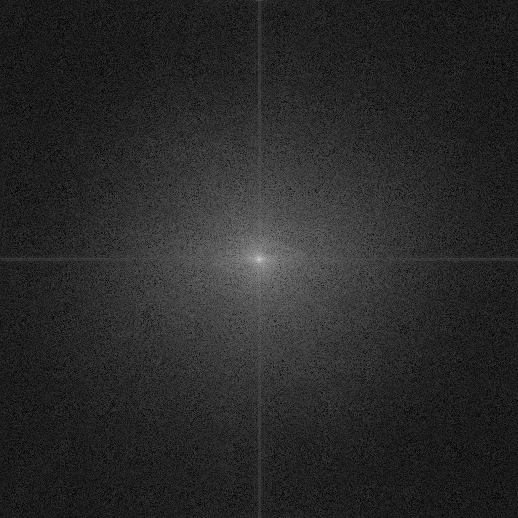
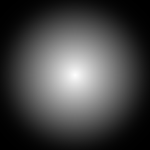
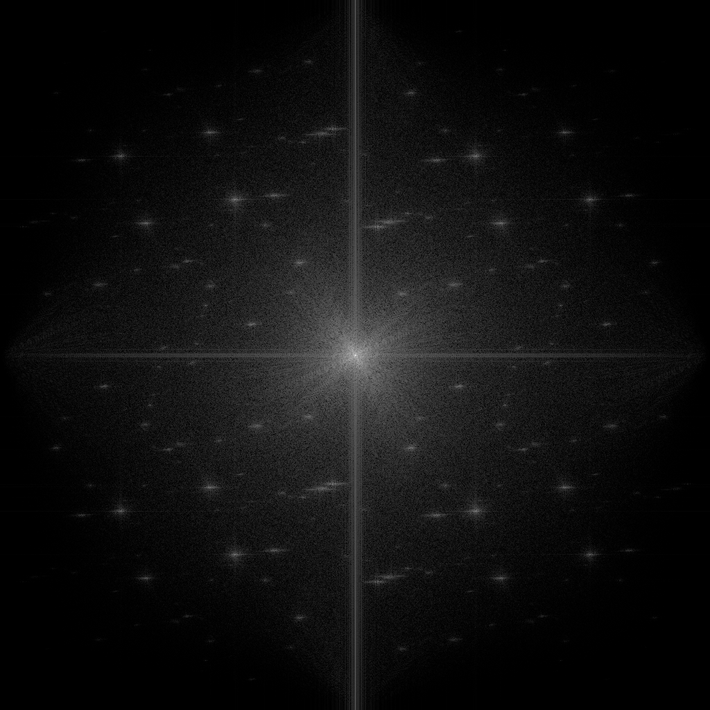
For the theoretical analysis of the performance of the filters, we have to assume something about the distribution of the image energy on the frequency domain. I'll analyze two assumptions: uniform distribution, which is in a sense the worst-possible case in terms of in-spectrum loss and aliasing possibilities, and exponential distribution from the center, which seems to be much better for the performance of filters, and also closer to real-life images. As a matter of fact, power spectra of real photographs do resemble exponential distributions 9 10 11 12. Remember that the visualizations of power spectra are on the log domain, so linear tendencies in the visualization indicate exponential growth. A near- uniform distribution of frequencies was only experienced in the zone-plate image.
To evaluate the performance, we compute the integrals of the power
spectra of the original image (in this case, the expected
distribution) and filtered ones. We also compute the integrals for the
in-spectrum (for both 2x and 4x subsampling) energies. The difference
between in-spectrum energies of original and filtered gives the
in-spectrum loss, while the difference between energies outside of the
spectrum and the total filtered ones give the foldback. The
exponential distribution gives an energy of ![]() , and the
domain
, and the
domain ![]() .
. ![]() is the distance from the center of the domain.
is the distance from the center of the domain.
The interesting thing to notice is that the zone plate image is performing close to its theoretically worse. This supports the argument that it is the ideal image for testing filtering techniques at the worst possible conditions. At the same time, we can compare it to real-life images, and even with relatively pathological images such as Figure 8, the in-spectrum loss and foldback are not too bad. This seems to indicate that our test is overly harsh.
It seems my exponentially decreasing power spectra does not match exactly the images. For one, the in-spectrum loss expected is still larger than the ones experienced. Still, it does seem to predict the small amount of leaked energies in real images as the experiments showed.
I think it is possible to design optimal filters, similar to the Wiener sense that will minimize both foldback and in-spectrum noise, assuming we know the spectra of the images. Since it seems that an exponentially decreasing power spectrum is at least somewhat appropriate for real-life images, this could give optimal filters for a certain subsampling.
In this next section, I investigated interpolating filters for supersampling. Specifically, I implemented sinc reconstruction (by padding in the Fourier domain), nearest-neighbor and bilinear (on the spatial domain).
The first interpolating filter works in the fourier domain. By padding the fourier domain with extra zeros, we are effectively multiplying the original image by a rectangle function on a larger domain. The inverse fourier transform of this is a convolution of the original function by a sinc function of period equal to the original resolution. The pixels that are between the original samples are the reconstructed with the sinc interpolation.
In theory, sinc interpolation is the best possible interpolation scheme, because no new frequencies are introduced (by definition). The problem that arises in practice is that similar artifacts to the ideal low-pass filters appear: sinc reconstruction near sharp edges cause ringing.
The following filters work in the spatial domain and they give visually better results. On the other hand, they have definite effects on the Fourier domain, as we'll see.
The next filter I investigated is the nearest-neighbor filter. With 2x supersampling, this is equivalent to convolving the image with a box filter two pixels thick. On the frequency domain, this is equivalent to multiplying with a sinc filter of period 1/2. But since we're increasing the domain to twice the size, we're going to see the frequency domain repeated. So there will be multiple copies of noise artifacts on the resulting domain, and they will be damped only slightly, because the sinc function decreases slowly.

 |
 |
The code I used for this assignment is included in the directory code. It is basically a mish-mash of VISPack code for the filtering peppered with many bash scripts to automate the job. I used ImageMagick to convert FITS images to PNGs.
Whew! This was a lot of work. But at the same time, it was really cool to see the artifacts of sampling and how periodic noise shows up on the Fourier Domain. I feel I learned a lot. I apologize for the extremely late submission.
This document was generated using the LaTeX2HTML translator Version 2002 (1.62)
Copyright © 1993, 1994, 1995, 1996,
Nikos Drakos,
Computer Based Learning Unit, University of Leeds.
Copyright © 1997, 1998, 1999,
Ross Moore,
Mathematics Department, Macquarie University, Sydney.
The command line arguments were:
latex2html index.tex -split 0 -nonavigation
The translation was initiated by Carlos Scheidegger on 2005-05-04