


Gamma correction is normally used to correct the non-linear response of CRT displays. In CRT's, intensity curves like this

are displayed like this:

This distorition is usually modeled by a power law: displayed_image = image ^ gamma. In order for CRT's to display accurate intensity curves, we need to compensate this, and this is usually called gamma correction. Since this transformation effectively shrinks some parts of the intensity curves and expands others, we can also use this technique to bring out details in lower or higher intensities.
I used gamma correction to try to adjust the following images. I ran my program to create 30 different gamma-corrected images, with gamma varying from 0.1 to 3.0. All of the images generated are in this directory. Here, we'll show some typical examples of the results that can be obtained.

This transformation, with gamma=0.5, shrinks the dark side of the intensity curve, and so things that are darker appear brighter. The result is that we are now able to see the person in the picture much better than before. Obviously the brighter areas lose contrast (for example, the mountains), because of the reduced "intensity real estate". In case we want to discern more things in the bright areas, we can use gammas larger than 1. For example, the following image has gamma=3.0:

Now the person in the picture is completely lost, but we are able to discern more details in the bright areas, such as the change in sky intensities, the "A" permit sign, and the mountains.

The previous images show the original image transformed by gammas respectively of 0.5, 3.0 and 6.0. Notice that neither of them seems to improve the image significantly. I think this happens because there is not enough range for the compression and expansion of the intensity range of gamma correction to work. If we were allowed to expand the range of image, the results would look much better.

The previous images show the original image transform by gammas respectively of 0.5, 2.0 and 3.0. The first image looks significantly better than the other two: That's because most of our interesting features, just like in image 1, are in the darker areas. A gamma less than one will expand the dark portion of the intensity curve, and a gamma more than one will expand the brighter portion. That's the reason the gammas of 2.0 and 3.0 do not help in this case (except for bringing out the curtain fabric details).
Histogram equalization is a technique that aims to maximize the "information efficiency" of the image, in the sense that more frequent pixels should be entitled to a larger intensity range. Surprisingly, the function that does this transformation is the cumulative distribution function of the image histogram. I implemented this technique for the following images:
| Untransformed image | transformed image |
|
|
|
|
|
|
|
|
|
|
|
|
The first image, xinwei1.tif, doesn't give us the desired results because the person area relative to the lawn area in the picture is too small. The effect this has is that the shadows of the trees on the lawn become enhanced, but the person isn't helped much. Also, since there is no geometric information on the H.E., we can see some artifacts on the person's face related to the fact that that intensity of gray is found in other places in the picture.
The second image, xinwei2.tif, is an attempt to mitigate the previously described problem, by cropping the lawn out and equalizing the histogram only on the ROI. This does enhance the contrast, but introduces noise because of the limited range in the ROI.
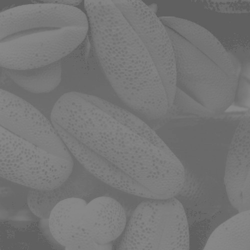
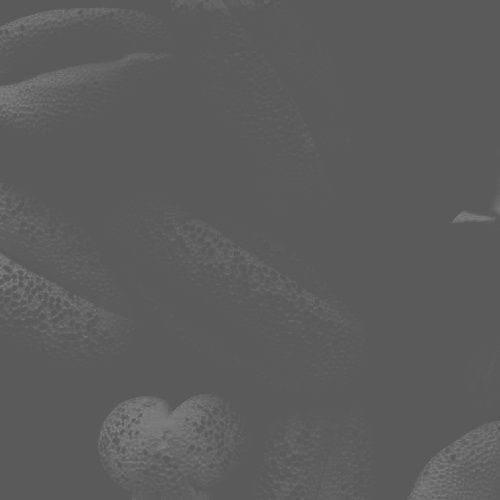
The third image, seeds.jpg, is dramatically improved. This is the same image in which gamma correction failed to improve the quality. I speculated that lack of range could be the cause, and although this doesn't necessarily show that to be the case, we see that with an increased range, we can see the lattice-like features on the seeds much better, because they account for much of the pixel area in the image, and so they get a large range.
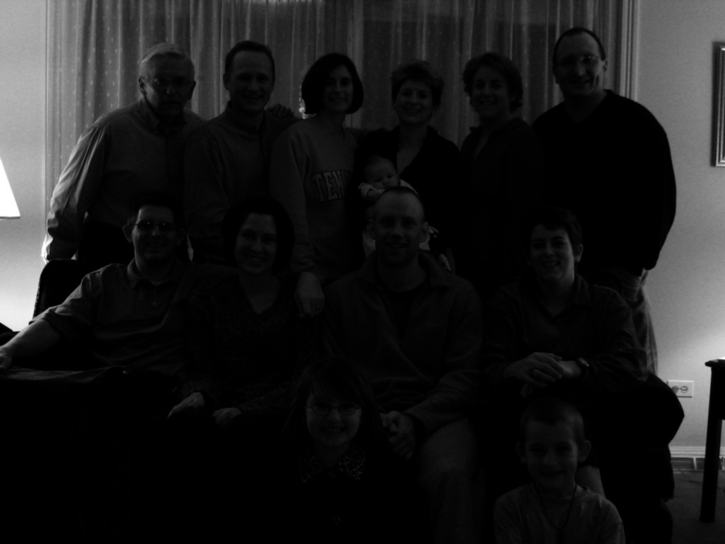
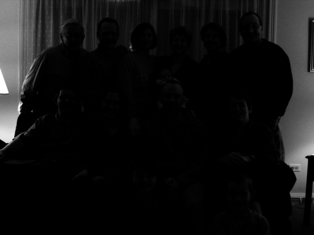
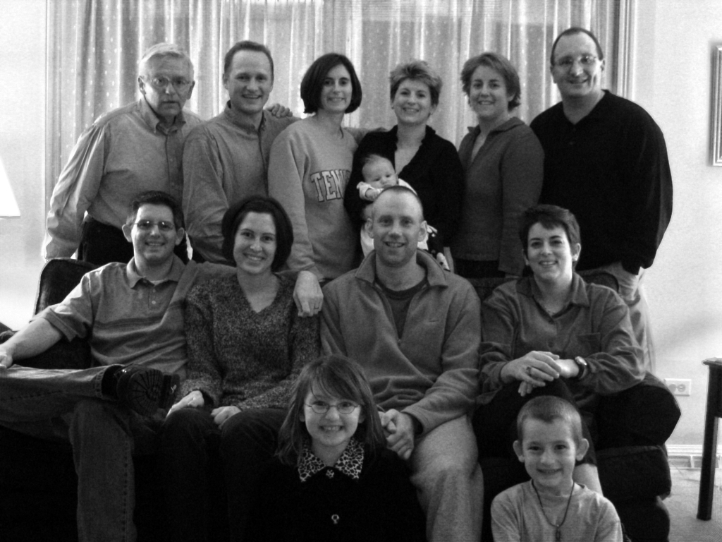
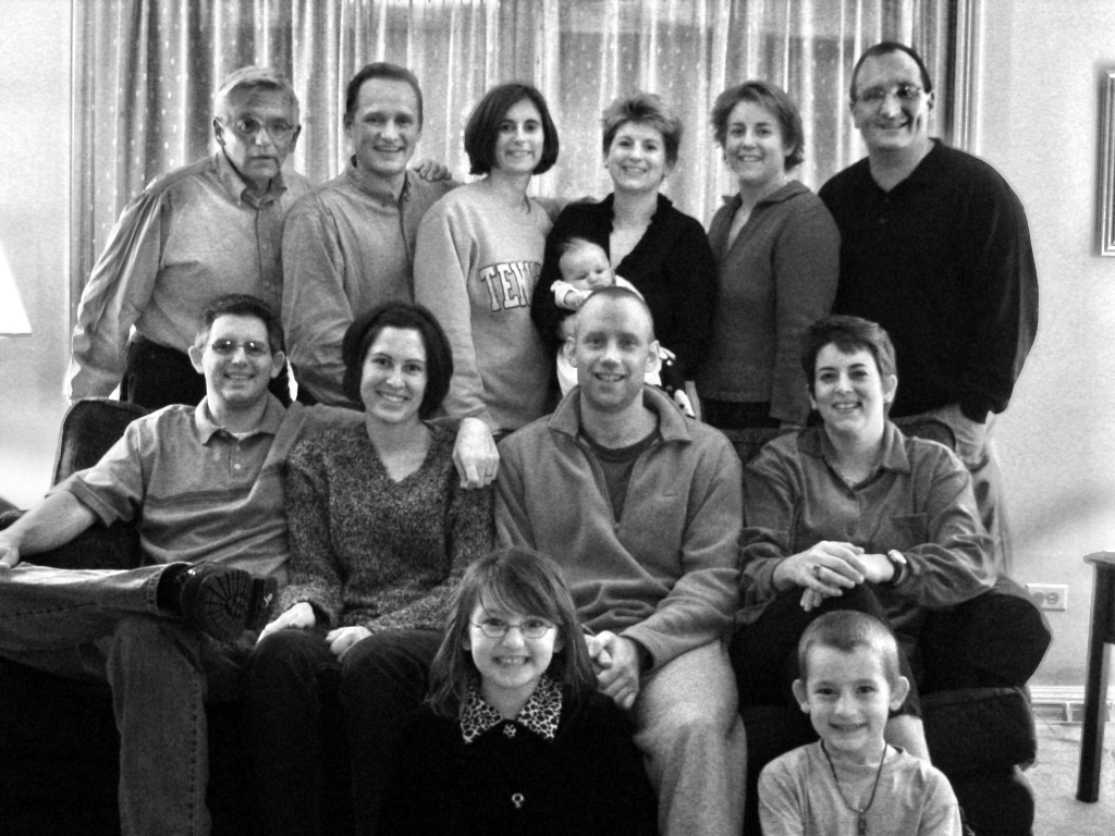
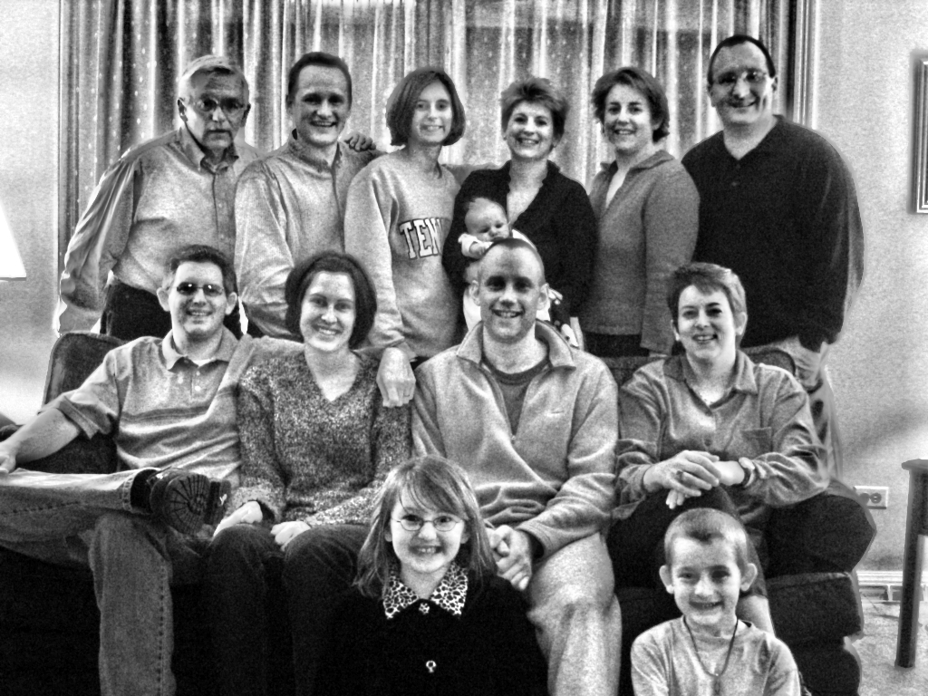
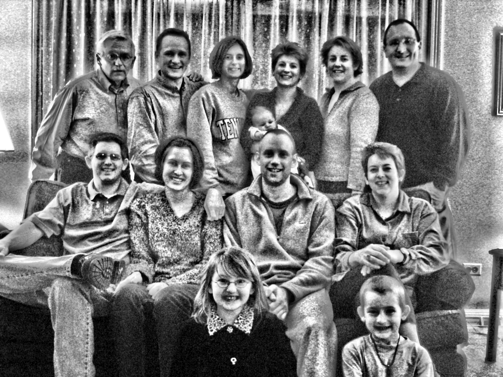
The fourth image, family.tif, is also improved, but a significant amount of noise is introduced, specially in the darker areas. This is because although the dark areas are not our ROI, it accounts for a significant part of the image pixels.
capitol.jpg is improved (notice the window details next to the flag), but also with a considerable amount of introduced noise.
In the last image, portal.tif, we are supposedly interested in the bright areas. Unfortunately, the background has a significant area. Even though there isn't much noise introduced, the intensities in the background get stretched according to their area.
I would like to illustrate the effect of differing bin count has on histogram equalization. For this, I'll use family.tif, scaled down to a fourth of the original size only for visibility. | 1 bin |
 | 2 bins |
 | 4 bins |
 | 8 bins |
 | 16 bins |
 | 32 bins |
 | 64 bins |
 | 128 bins |
 | 256 bins |
| Original image |
| HE of original image |
 | CL HE of original image, max_slope=2 |
 | CL HE of original image, max_slope=3 |
I've implemented both the window-based and tile-based AHE. The window-based AHE gives much better results as we'll see, and can be made asymptotically as efficient as the tile-based AHE, as will be explained.
For the window-based AHE, my algorithm to choose the window size was to take the square root of the smaller dimension, and use that as the radius of the neighborhood. This was based on the observation that the original algorithm takes n^2 neighborhoods, and if each neighborhood is of size m, the total complexity is O(n^2 m^2). If we assume that computing the CDF is O(1) (which is not true), setting m=sqrt(n) lets us at least predict the total complexity of the algorithm to be O(n^3).
The first improvement to the window-based algorithm takes advantage of the coherence of the histogram between neighbors. Noticing that after initializing the histogram, updating the histogram from one neighbor to another takes O(m) time, the total time is already reduced to O(n^2.5).
If we're willing to raise our memory consumption from O(m^2) to O(nm), there's an algorithm that takes O(n^2) time. The idea is to keep a 1D histogram of each vertical neighborhood of a horizontal line. This allows us to update each of these neighborhoods with O(1) operations (remove the top element, then add the bottom one). Since we have O(n) of these histograms, and we have to update each of them O(n) times, it's O(n^2) total. I haven't implemented this last improvement, because I couldn't see how to build CDF's in O(1) or even in O(m) time. This means that the original complexity is O(n^2 (n + n)), and each of the improvements only brings us to O(n^2 (sqrt(n) + n)) and O(n^2 (1 + n)), all of them being O(n^3). It isn't practical, then, to implement it. I implemented the first optimization before noticing the hidden costs of the CDF creation.
These tests were run on a 1GHz G4 iBook with 768MB RAM. Columns show different window sizes, times are in seconds.
Each file name links to the directory with all of the files.| File name | 2 | 4 | 8 | 16 | 32 | 64 | 128 |
| xinwei1.tif | 43.5s | 44.7s | 47.1s | 51.9s | 60.9s | 75.4s | 97.4s |
| xinwei2.tif | 30.4s | 31.2s | 32.8s | 36.3s | 41.9s | 50.8s | 62.9s |
| family.tif | 163.5s | 168.9s | 178.2s | 196.2s | 231.3s | 299.6s | 435.4s |
| capitol.jpg | 33.8s | 34.7s | 37.1s | 40.5s | 47.4s | 58.7s | 72.2s |
| portal.tif | 18.0s | 18.4s | 19.5s | 21.5s | 24.9s | 29.5s | 33.6s |
| seeds.jpg | 50.2s | 52.3s | 55.1s | 60.5s | 70.7s | 88.3s | 113.7s |
As the window size increases, we seem to be getting quadratically slower, because the complexity is O(n^2 m^2), and m is increasing.
The first thing we can notice is that AHE is very sensible to the window size. When the window size is approximately the size of an "interesting feature", we get an ideal contrast enhancement. Notice the faces of the people in family.tif, xinwei1.tif and xinwei2.tif. If the feature size is underestimated, we get pure noise. If the feature size is overestimated, we get banding because of "mixing histograms". I wonder if our vision mechanism does something similar, and if that's the reason for our perception of decreasing bands in ladder-like greyscale images. Notice the two images:
 | Mach bands - all bands are the same color, but they appear to be different |
 | AHE of the above image, window size 64. Now the image itself is banded, reflecting our illusions. |
For the tile-based AHE, we compute tile_x*tile_y histograms and interpolate between the equalized values as given from the four neighboring CDF's at each time. Since the running time is O(time_to_compute_CDFs + n^2), and time_to_compute_CDFs is O(tile_x*tile_y*time_to_compute_each_CDF). Since time_to_compute_each_CDF = (width/tile_x)*(height/tile_y), time_to_consume_CDFs is O(width*height) = O(n^2), so, surprisingly, the running time is always going to be O(n^2), regardless of the number of tiles. This was confirmed by the fact that the run times didn't change for runs of the same image and different tile counts.
Again, we can see that AHE is very sensible to the window (in this case, tile) size. Also, tile-based AHE has the additional problem that unless the tile splits are placed on "good" positions, we'll get unexpected bleeding and interactions between two different histograms.
Each directory contains files {1,2,3,5,8,11}.jpg. Each of these files correspond to the image corrected with CLAHE with default window size and given max_slope:
The following images are the sequence of max_slopes = {1,2,3,5,8,11} for family.tif:


CLAHE seems to be much more effective at raising local contrast without actually blowing up the noise. Notice the difference in the darker areas: the limit in contrast change do prevent the noise to become a serious issue. Values between 2 and 3 seem to give the best contrast enhancement without overly compromising the image quality. Values less than that give results too close to the original image (since the CDF is close to being an identity transformation), and values more than that give images that simply resemble AHE.