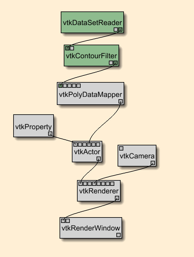
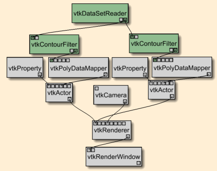
In this part of the project, we want to extract meaningful isosurfaces from a portion of the Visible Human dataset. To do that, we'll use the vtkContourFilter class from VTK. The first part of the project is to actually determine the interesting isosurfaces. I found two of them: one roughly related to the skin of the model, and one roughly related to the bones. One way of determining these automatically is using techniques like the Contour Spectrum, in which differential quantities of isovalues are computed and local maxima tend to indicate more interesting isovalues. Since VTK does not offer any similar technique, I resorted to experimentation. For that, I used a recently published system called VisTrails [1], which offers a visual dataflow programming paradigm similar to SCIRun [2], and has VTK as the underlying computational infrastructure. VisTrails was built to support comparative, multiview visualization, and explorations like these are particularly well-suited. Here's a figure of the dataflow used to explore the isosurface values:
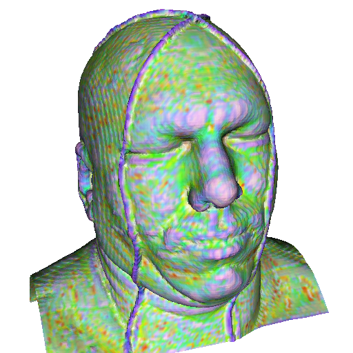
To find the best isosurface corresponding to skin, I experimented around the isovalue 25-50:
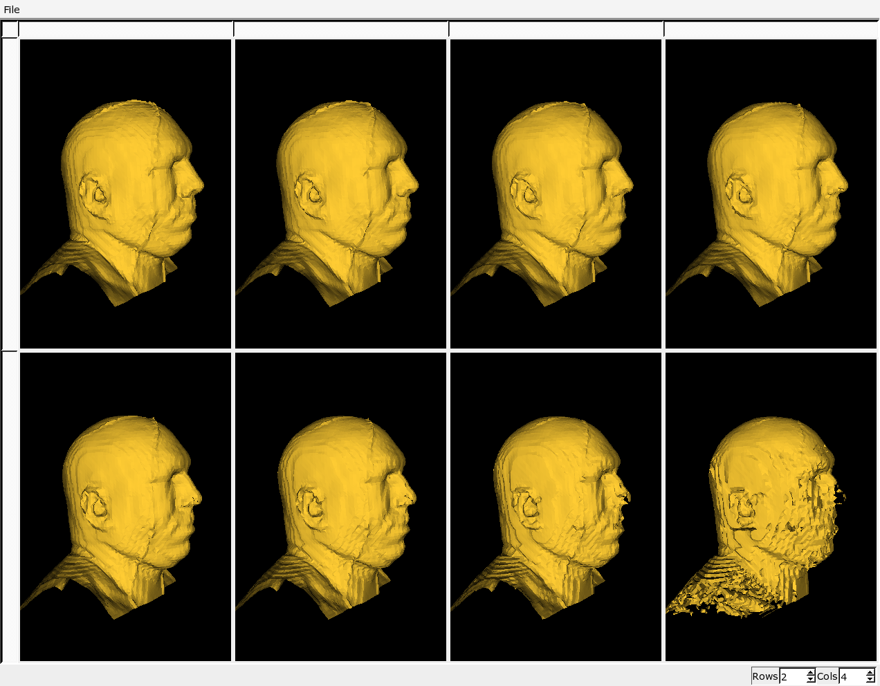
I found the best-looking iso-value for skin to be the value 30, in which details of the ear are still present. I could not remove the strange lines going through the head by changing the isovalue without seriously deteriorating the overall result (as can be seen on the lower row).
The second interesting isosurface is the one that shows the bone structure of the Visible Human. By looking around somewhat randomly, I found that the bone was somewhere between the values 60-120. The dataflow used was the same, with the exception that I now changed the diffuse coilor to off-white:
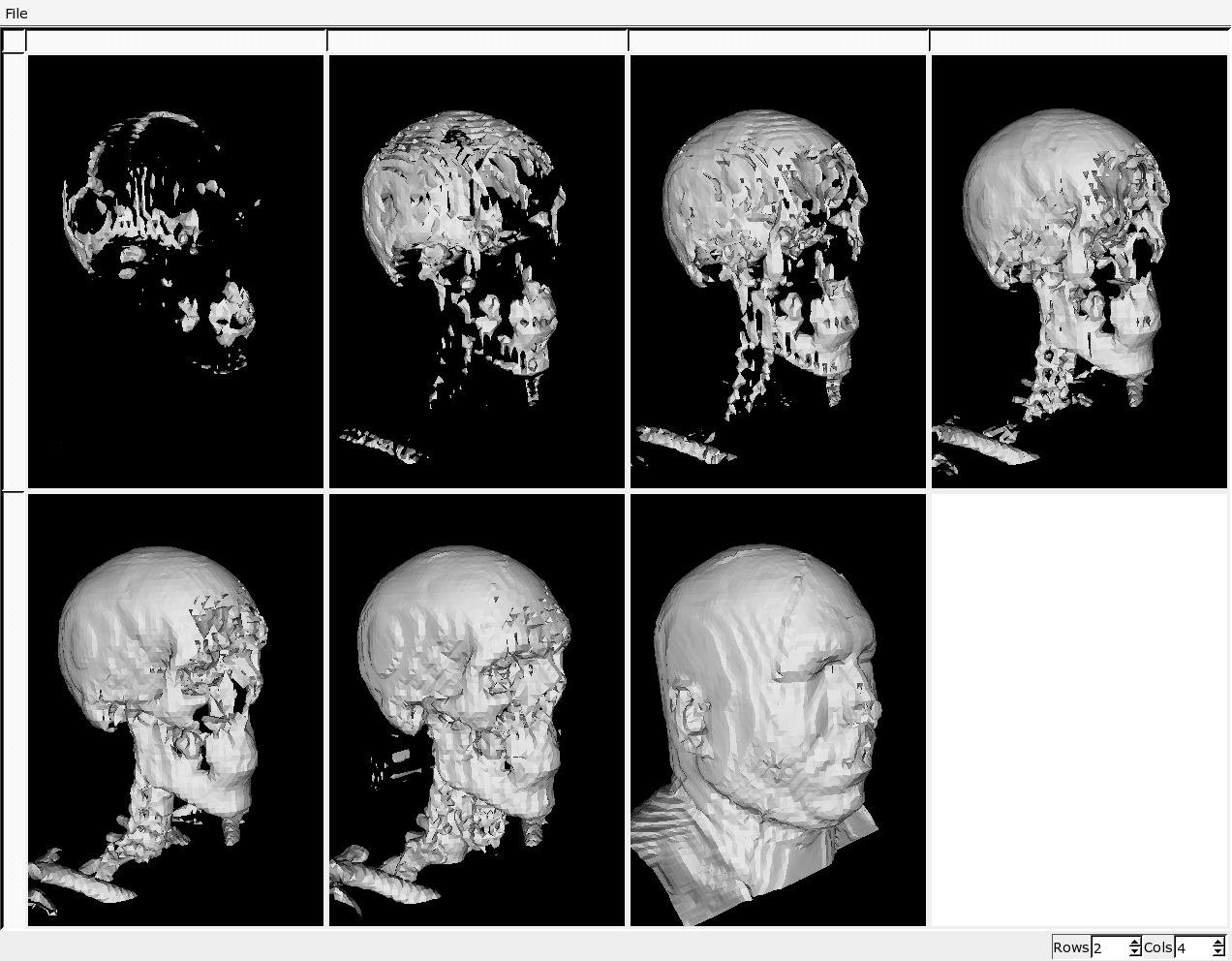
Each different view has a difference of 10 in the isovalue. The best isovalue seems to be between 70 and 80, so I decided to refine the search, to resolve the forehead bone structure (as in the second view from the lower row), but without the artifacts (as in the first view from the lower row). Another series of views shows the differences:
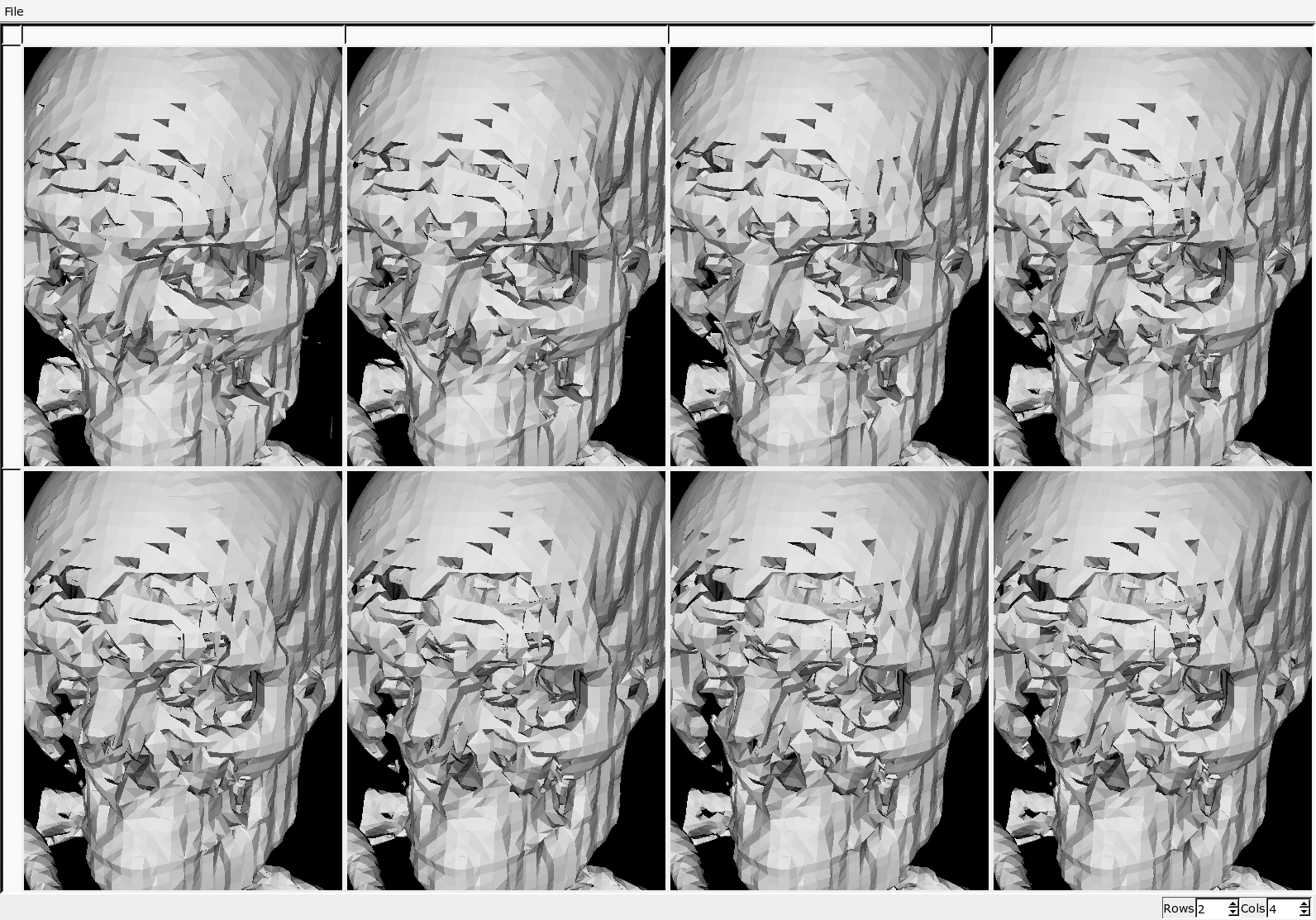
Again, somewhat arbitrarily I decided that the best-looking isosurface is the top-most in the right, since it exhibits no "floating" parts of bone, and still shows a resemblance of the forehead bone structure. Since I used the low-res version of the dataset to explore, I decided to compare it against the high-quality version. Again I set up a VisTrails multi-view window to see the results:
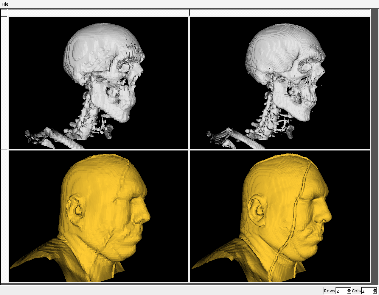
The high-res versions are shown in the right column, and it's clear that there's much more detail. At the same time, the choice of isosurface still seems to be appropriate.
if { [catch {set VTK_TCL $env(VTK_TCL)}] != 0} { set VTK_TCL ".." }
if { [catch {set VTK_DATA $env(VTK_DATA)}] != 0} { set VTK_DATA "../vtkdata" }

source "common.tcl"

# boilerplate stuff
proc connect { source oport dest iport } {
    $dest SetInputConnection $iport [$source GetOutputPort $oport]
}

set datasetresolution "60"
set bivariatecolormapresolution "8"
set datasetsuffix ".$datasetresolution.vtk"
set bivariatecolormapsuffix ".$datasetsuffix.$bivariatecolormapresolution.vtk"

# objects
vtkDataSetReader vh
vtkContourFilter bones
vtkContourFilter skin
vtkPolyDataMapper bonesMapper
vtkPolyDataMapper skinMapper
vtkProperty skinProperty
vtkProperty bonesProperty
vtkActor skinActor
vtkActor bonesActor
vtkCamera camera
vtkRenderer ren
vtkRenderWindow renwin
vtkRenderWindowInteractor iren
vtkInteractorStyleTrackballCamera trackball

# parameters
vh SetFileName "$VTK_DATA/head$datasetsuffix"
skin SetValue 0 30
bones SetValue 0 73
skinProperty SetDiffuseColor 1 0.8 0.2
skinProperty SetOpacity 0.5
bonesProperty SetDiffuseColor 0.8 0.8 0.8
bonesMapper ScalarVisibilityOff
skinMapper ScalarVisibilityOff
ren SetBackground 1 1 1
renwin SetSize 512 512

# dataflow topology
connect vh 0 skin 0
connect vh 0 bones 0
connect skin 0 skinMapper 0
connect bones 0 bonesMapper 0

# object topology
skinActor SetMapper skinMapper
skinActor SetProperty skinProperty
bonesActor SetMapper bonesMapper
bonesActor SetProperty bonesProperty
ren SetActiveCamera camera
ren AddActor skinActor
ren AddActor bonesActor
iren SetRenderWindow renwin
iren SetInteractorStyle trackball
renwin AddRenderer ren

# More boilerplate
iren Initialize
ren ResetCamera
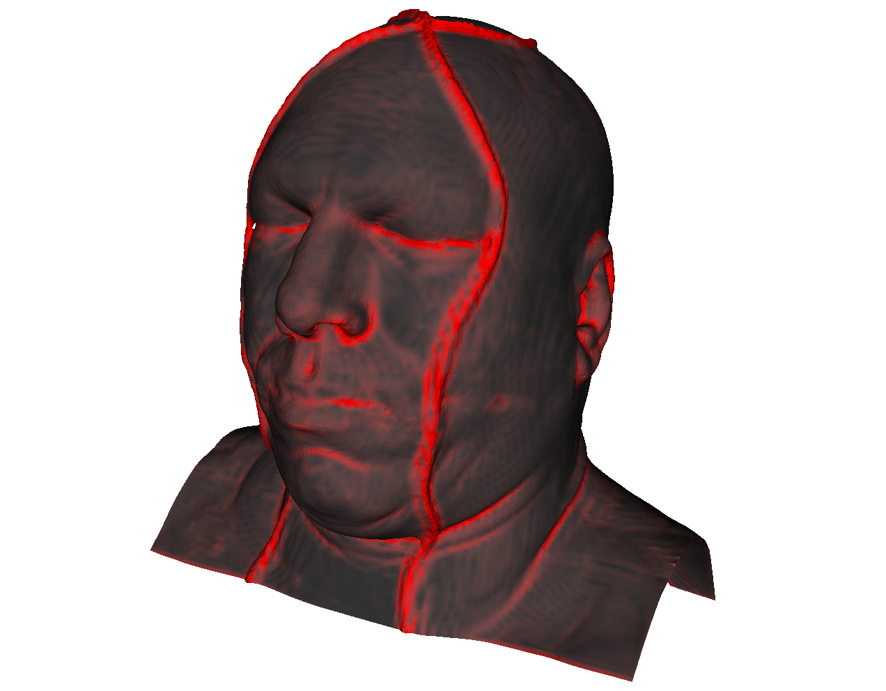
In the second part of the project, we want to display both isosurfaces together. So that the user can see both of them, the skin will not be completely opaque. The dataflow used for this visualization is shown on the next figure:
To investigate the best-looking opacity, I set up four different views whose only changed parameter was the opacity:
The best-looking visualization seems to be the top-right one, where both isosurfaces can be seen clearly. It is the one where the opacity is set at 0.5. With that in mind, I implemented the code in TCL as shown in the right column.
if { [catch {set VTK_TCL $env(VTK_TCL)}] != 0} { set VTK_TCL ".." }
if { [catch {set VTK_DATA $env(VTK_DATA)}] != 0} { set VTK_DATA "../vtkdata" }

source "common.tcl"


# boilerplate stuff
proc connect { source oport dest iport } {
    $dest SetInputConnection $iport [$source GetOutputPort $oport]
}

set curvaturename "norm"
set datasetresolution "120"
set bivariatecolormapresolution "8"
set datasetsuffix ".$datasetresolution.vtk"
set bivariatecolormapsuffix ".$datasetsuffix.$bivariatecolormapresolution.vtk"


# objects
vtkDataSetReader vh
vtkContourFilter skin
vtkSmoothPolyDataFilter smooth
vtkDataSetReader curvature
vtkProbeFilter probe
vtkPolyDataMapper skinMapper
vtkProperty skinProperty
vtkActor skinActor
vtkCamera camera
vtkRenderer ren
vtkRenderWindow renwin
vtkRenderWindowInteractor iren
vtkLookupTable table
vtkInteractorStyleTrackballCamera trackball


# parameters
vh SetFileName "$VTK_DATA/head$datasetsuffix"
smooth SetNumberOfIterations 2
smooth SetRelaxationFactor 0.5
skinMapper SetColorModeToMapScalars
skinMapper SetScalarRange 0 128
curvature SetFileName "$VTK_DATA/$curvaturename$datasetsuffix"
skin SetValue 0 30
ren SetBackground 1 1 1
renwin SetSize 512 512
table SetHueRange 0.0 0.0
table SetSaturationRange 0.0 1.0
table SetValueRange 0.3 1.0

# dataflow topology
connect vh 0 skin 0
connect skin 0 smooth 0
connect smooth 0 probe 0
connect curvature 0 probe 1
connect probe 0 skinMapper 0

# object topology
skinActor SetMapper skinMapper
skinMapper SetLookupTable table
ren SetActiveCamera camera
ren AddActor skinActor
iren SetRenderWindow renwin
iren SetInteractorStyle trackball
renwin AddRenderer ren

# More boilerplate
iren Initialize
ren ResetCamera
if { [catch {set VTK_TCL $env(VTK_TCL)}] != 0} { set VTK_TCL ".." }
if { [catch {set VTK_DATA $env(VTK_DATA)}] != 0} { set VTK_DATA "../vtkdata" }

source "common.tcl"


# boilerplate stuff
proc connect { source oport dest iport } {
    $dest SetInputConnection $iport [$source GetOutputPort $oport]
}

set curvaturename "angle"
set datasetresolution "120"
set bivariatecolormapresolution "8"
set datasetsuffix ".$datasetresolution.vtk"
set bivariatecolormapsuffix ".$datasetsuffix.$bivariatecolormapresolution.vtk"


# objects
vtkDataSetReader vh
vtkContourFilter skin
vtkSmoothPolyDataFilter smooth
vtkDataSetReader curvature
vtkProbeFilter probe
vtkPolyDataMapper skinMapper
vtkProperty skinProperty
vtkActor skinActor
vtkCamera camera
vtkRenderer ren
vtkRenderWindow renwin
vtkRenderWindowInteractor iren
vtkLookupTable table
vtkInteractorStyleTrackballCamera trackball


# parameters
vh SetFileName "$VTK_DATA/head$datasetsuffix"
smooth SetNumberOfIterations 2
smooth SetRelaxationFactor 0.5
skinMapper SetColorModeToMapScalars
skinMapper SetScalarRange 0 255
curvature SetFileName "$VTK_DATA/$curvaturename$datasetsuffix"
skin SetValue 0 30
ren SetBackground 1 1 1
renwin SetSize 512 512

# dataflow topology
connect vh 0 skin 0
connect skin 0 smooth 0
connect smooth 0 probe 0
connect curvature 0 probe 1
connect probe 0 skinMapper 0

# object topology
skinActor SetMapper skinMapper
skinMapper SetLookupTable table
ren SetActiveCamera camera
ren AddActor skinActor
iren SetRenderWindow renwin
iren SetInteractorStyle trackball
renwin AddRenderer ren

# More boilerplate
iren Initialize
ren ResetCamera
The third part of the assignment required us to visualize the curvature volumes provided by using the vtkProbeFilter class along with an appropriate colormap. I again used VisTrails to explore the parameter space. The dataflow is as follows:
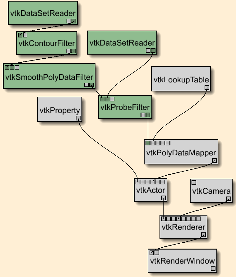
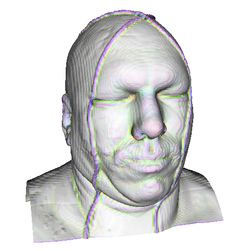
Notice that I added an additional smoothing step after the isocontour extraction. The reason I did this was so that the resulting triangles were nicer. Particularly, the shading becomes much smoother and it's then easier to determine the different curvature values. In these figures you can see the difference:

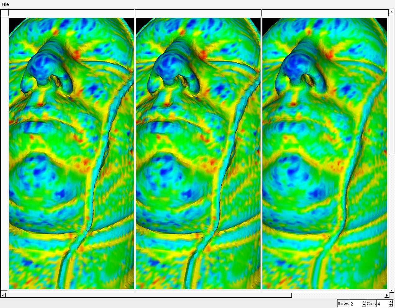
To decide on the best colormap to visualize the norm of the curvature, I used VisTrails, where I could directly compare a series of different colormaps side by side. This is a screenshot of the session:

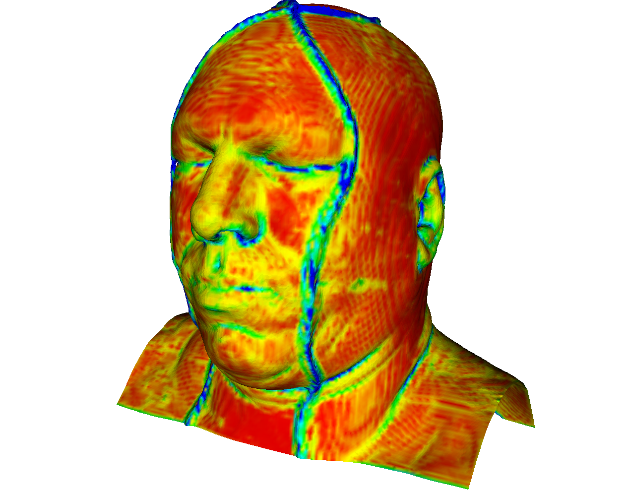
The top row shows how bad it is to use different hues for the total curvature. This is because different hues are best used to visualize scalars in which there's no relation between different scalars - the colormap is simply used for differentiation. Since we want to be able to notice higher total curvature, hue is not really appropriate. I decided to use a combination of value and saturation on a red hue:
We can see clearly with this colormap that the norm of the second fundamental form gives a clear indication of the total amount of curvature (how much the surface fails to be a plane). If we had used a hue-based colormap, it would have been harder to tell which parts of the surface are more bent:
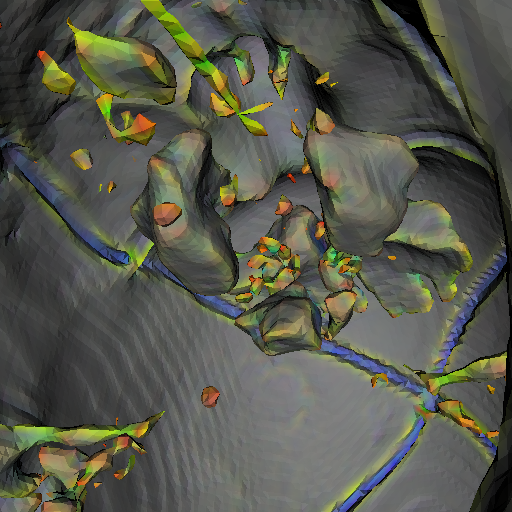
The next curvature invariant we want to visualize is the trace. The trace gives an overall idea of the shape of the surface. The default colormap for VTK uses hue, and since we don't want to perceive one shape as "more" or "less" than the other, hue variation is an adequate choice for this colormap:
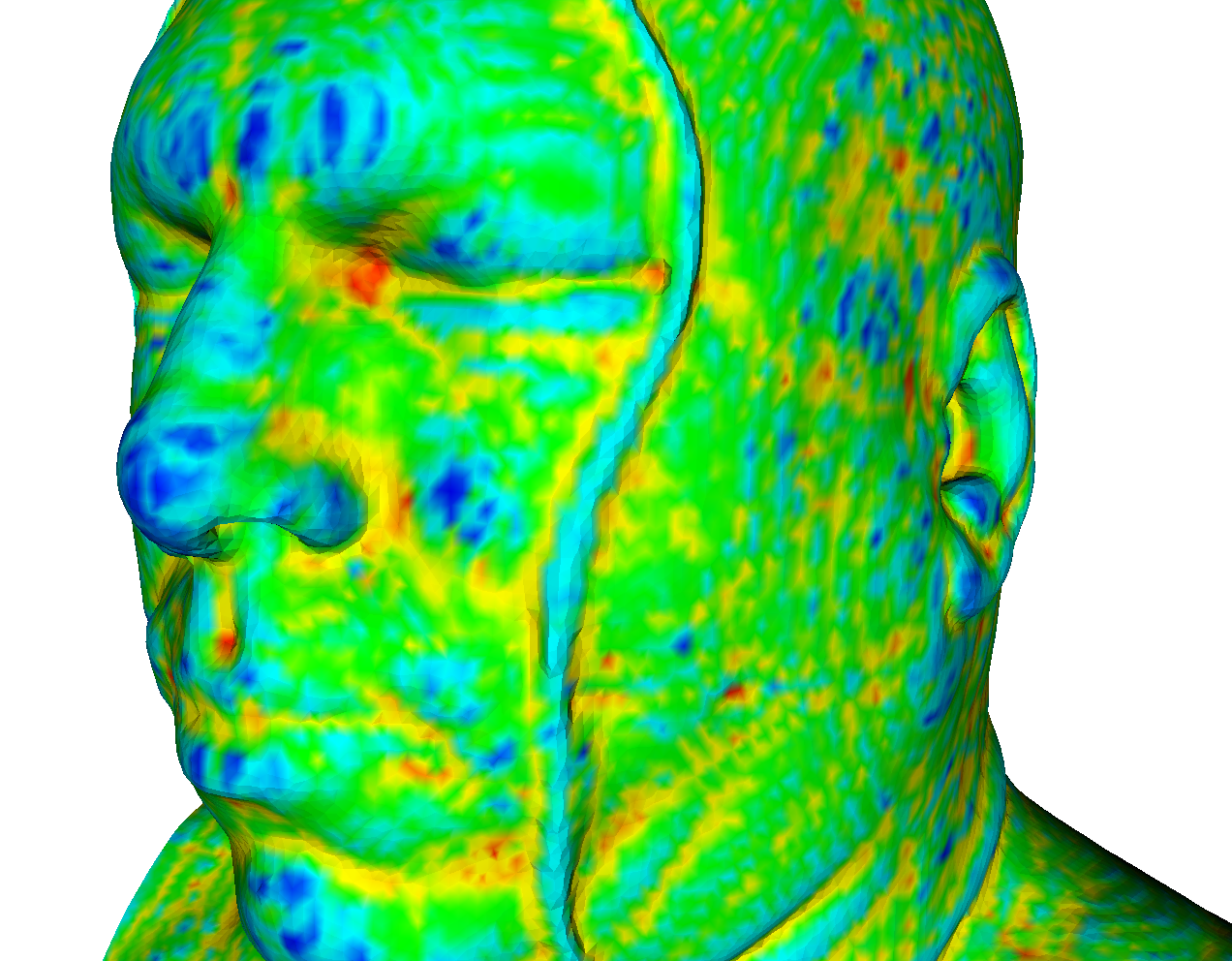
Hue is indeed a good indicator: notice how peaks are blue, ridges are cyan, saddle regions are green, valleys are yellow, and bowls are red. If we had used value or saturation, it would have been hard to discriminate the different regions:

if { [catch {set VTK_TCL $env(VTK_TCL)}] != 0} { set VTK_TCL ".." }
if { [catch {set VTK_DATA $env(VTK_DATA)}] != 0} { set VTK_DATA "../vtkdata" }

source "common.tcl"

proc ValueHueSaturation { lut pos x y res } {
    global mnh
    global mns
    global mnv
    global mxv
    global mxh
    global mxs
    set h [clamp $y $mnh $mxh]
    set s [clamp $x $mns $mxs]
    set v [clamp $x $mnv $mxv]

    set i [expr int($h * 6.0)]
    set f [expr ($h * 6.0) - $i]

    set p [expr $v * (1 - $s)]
    set q [expr $v * (1 - ($s * $f))]
    set t [expr $v * (1 - ($s * (1 - $f)))]

    switch $i {
	0 { $lut SetTableValue $pos $v $t $p 1 }
	1 { $lut SetTableValue $pos $q $v $p 1 }
	2 { $lut SetTableValue $pos $p $v $t 1 }
	3 { $lut SetTableValue $pos $p $q $v 1 }
	4 { $lut SetTableValue $pos $t $p $v 1 }
	5 { $lut SetTableValue $pos $v $p $q 1 }
	default { $lut SetTableValue $pos $v $t $p 1 }
    }
}

proc makeBivariateLUT { lut res theproc } {
    $lut SetNumberOfTableValues [expr $res * $res]
    for {set x 0} {$x<$res} {incr x} {
	for {set y 0} {$y<$res} {incr y} {
	    $theproc $lut [expr $y * $res + $x] $x $y $res
	}
    }
    $lut SetTableRange 0 [expr $res * $res]
    $lut Build
}

set datasetresolution "120"
set bivariatecolormapresolution 8
set bivariatecolormapdim [expr int(pow(2, $bivariatecolormapresolution))]
set datasetsuffix ".$datasetresolution.vtk"
set bivariatecolormapsuffix ".$datasetresolution.$bivariatecolormapresolution.vtk"

set mns [expr  0.0 * $bivariatecolormapdim]
set mxs [expr  0.5 * $bivariatecolormapdim]
set mnh [expr  0.0 * $bivariatecolormapdim]
set mxh [expr  1.2 * $bivariatecolormapdim]
set mnv [expr -1.0 * $bivariatecolormapdim]
set mxv [expr  0.5 * $bivariatecolormapdim]

# objects
vtkDataSetReader vh
vtkContourFilter skin
vtkSmoothPolyDataFilter smooth
vtkImageMapToColors imageMapToColors
vtkDataSetReader curvature
vtkProbeFilter probe
vtkPolyDataMapper skinMapper
vtkProperty skinProperty
vtkActor skinActor
vtkCamera camera
vtkRenderer ren
vtkRenderWindow renwin
vtkRenderWindowInteractor iren
vtkLookupTable table
vtkInteractorStyleTrackballCamera trackball


# parameters
vh SetFileName "$VTK_DATA/head$datasetsuffix"
curvature SetFileName "$VTK_DATA/anglenorm$bivariatecolormapsuffix"
skin SetValue 0 30
ren SetBackground 1 1 1
renwin SetSize 512 512
makeBivariateLUT table $bivariatecolormapdim {ValueHueSaturation}

# dataflow topology
connect vh 0 skin 0
connect skin 0 smooth 0
connect smooth 0 probe 0
connect curvature 0 imageMapToColors 0
connect imageMapToColors 0 probe 1
connect probe 0 skinMapper 0


# object topology
imageMapToColors SetLookupTable table
skinActor SetMapper skinMapper
ren SetActiveCamera camera
ren AddActor skinActor
iren SetRenderWindow renwin
iren SetInteractorStyle trackball
renwin AddRenderer ren


# More boilerplate
iren Initialize
ren ResetCamera
One thing I noticed in this part of the assignment is that 6 bits for the entire range of the norm for the entire volume leads to severe quantization. Here's my colormap working on the 6-bit version:
Here's the colormap working on the 8-bit version:
The above figures show a preliminary colormap. Specifically, they use the entire range of the norm for the volume to colormap the data, which leads to the quantization artifact and to very washed-out colors because some small regions have very high curvature:
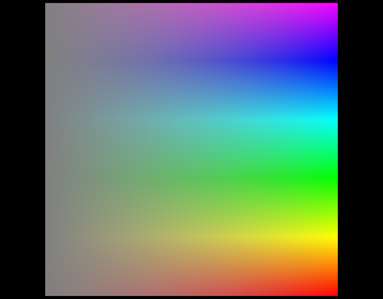
These features will push the highest curvature norm to a value that is usually not present in the isosurfaces, effectively reducing the dynamic range of the colormap. Since we're first colormapping and then probing the surface, it becomes impossible to figure out the minimum and maximum norms for a given surface. The solution is to manually clamp the ranges to an acceptable limit. The result is the following:
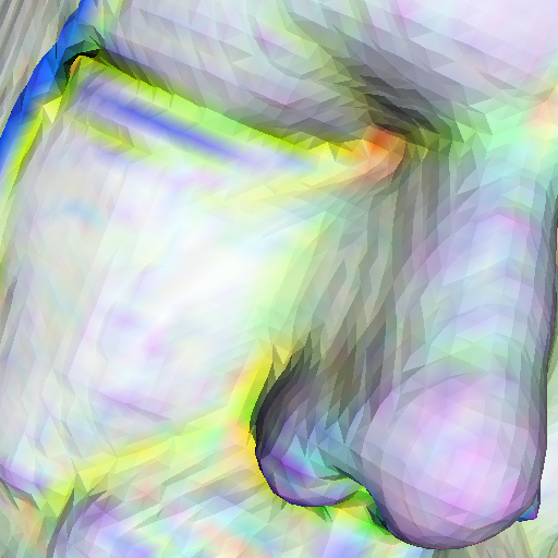
I also changed the hue slightly from the previous maps. Notice that in this figure we can clearly see the bivariate colormap working: In relatively flat regions, the colors are very washed out, making (as it should be) a very flat but valley-like region almost identical to a very flat but ridge-like region. In regions of high curvature, the saturation and value are higher, so the features are quite visible, like the red bowl in the inside of the eye, the yellow values tracing the face feature lines, the green saddles in the bridge of the nose, the purple peaks in the tip of the nose, and the blue ridges of whatever was surrounding the head at scan time. Notice that the higher curvatures stand out naturally.
I just noticed the scripts were supposed to be runnable in VTK 4.4, and VTK 4.4 does not use the new vtkAlgorithm based pipeline. I fixed my scripts so that they'd run on shell.cs.utah.edu, but the actual .tcl files are now different from the ones I show in this document.
[1] Bavoil, L. et al. VisTrails: Enabling Interactive Multiple-View Visualizations. In Proceedings of IEEE Visualization 2005.
[2] Parker, S. The SCIRun Problem Solving Environment and Computational Steering Software System, PhD Thesis, August 1999.