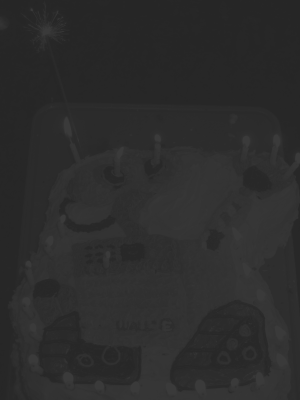
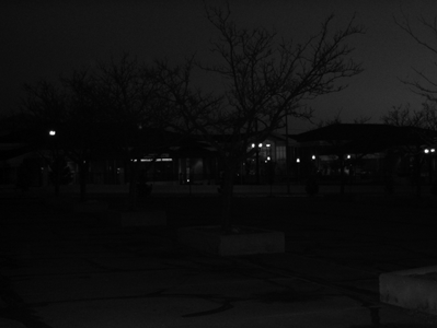
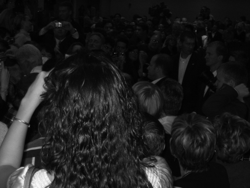
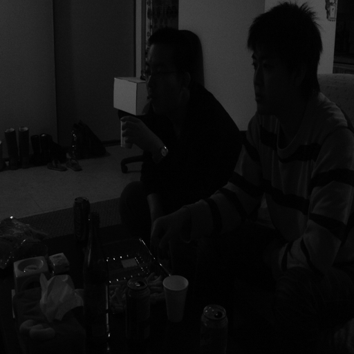
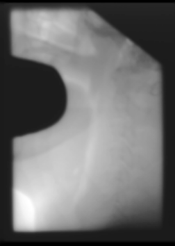
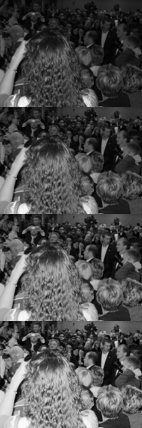
Original Image
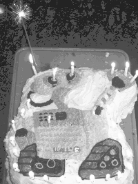
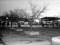
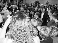
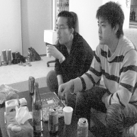
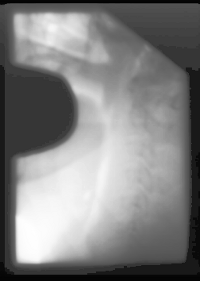
Equalized Image
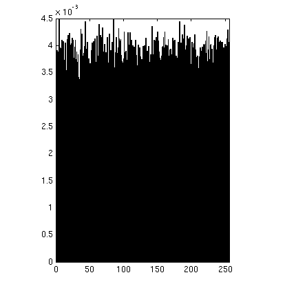
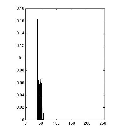
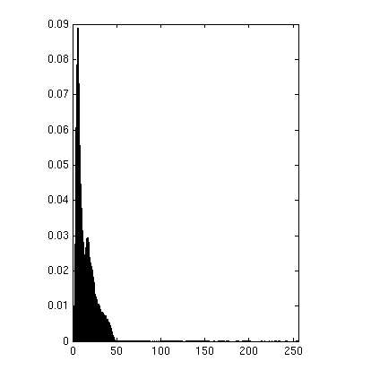
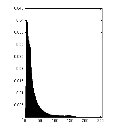
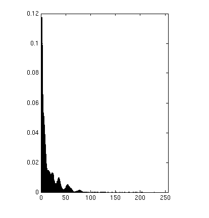
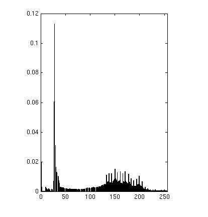
Original Histogram
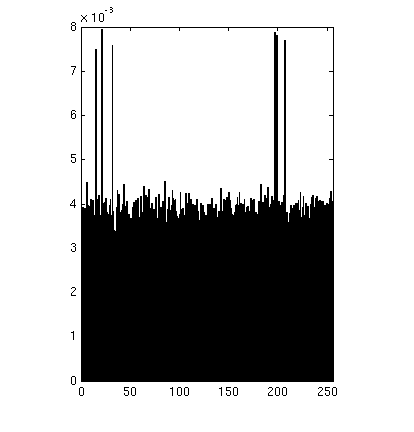
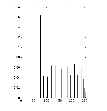
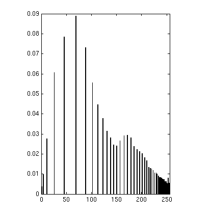
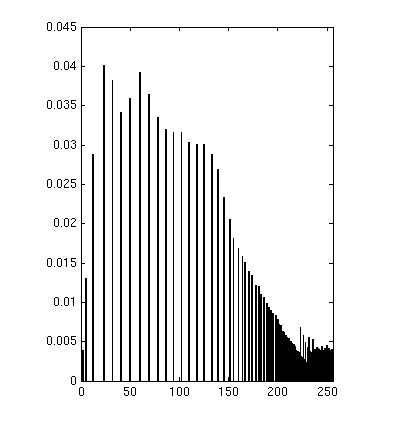
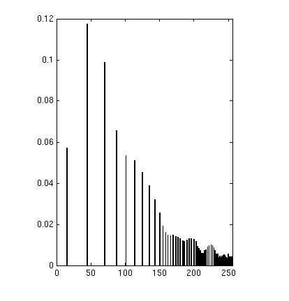
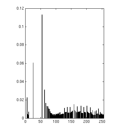
Equalized Histogram
Running time to equalize
0.0921 s
0.1824 s
0.3200 s
0.0603 s
Bradley C. Grimm
u0275665
snard6@gmail.com
Project 2
Note: I wrote a file Test_Project2.m that runs through all of the below tests and generates images (that can be clicked through) and also writes out images that can been viewed externally..
Throughout the project I used 7 different images. Four that were given in the assignment as well as three of my own. There is a large volume of images due to the nature of the assignment. Due to this large volume I will address an image (or set of the same image) per each section. The rest are supplied for reference. Also all of the images have been scaled down in size to save in the size of the report. To see these images, run the test suite and generate the images locally.
Histogram
Equalization
Matlab
Function: histogram.m histoeq.m
Part
1:
I took my implementation from last week and improved it to be
significantly faster. This modified implementation is found in
histogram.m.
Part
2:
My approach to the histogram equalization problem is found in
histoeq.m. I didn't do anything unique
here, I mostly followed the algorithm as specified. I generate a pdf
(histogram), build a cdf from that. And then scale the cdf by N-1.
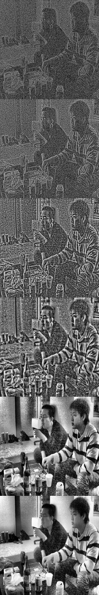
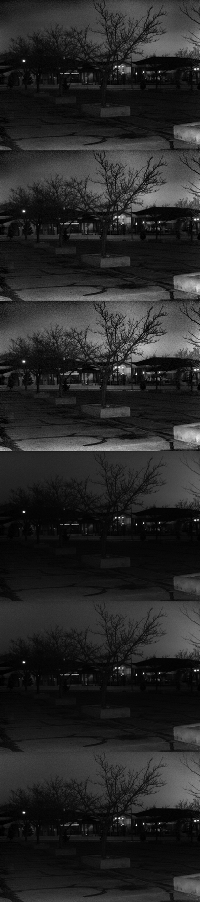
The result for the images was exactly as expected. For each of the
images we get a new image that visually is a lot easier to see. In
terms of the histogram, we notice it does what it can to flatten them
out.
Part 3 &
5:
Here are the examples for the images given to us as well as
some accompanying histograms:
|
Original Image |
Equalized Image |
Original Histogram |
Equalized Histogram |
Running time to equalize |
|
|
|
|
|
0.0921 s |
|
|
|
|
|
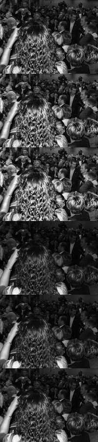
0.1824 s |
|
|
|
|
|
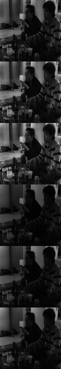
0.3200 s
|
|
|
|
|
|
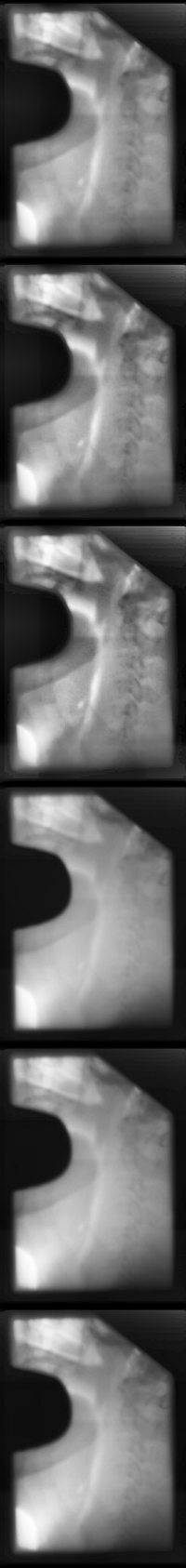
0.0603 s |
As we can
see, when there are large spikes of intensity the image can't break
them apart so it makes it hard to achieve a perfectly flat
histograms. But we do notice that it spreads them out a fair bit, and
uses the available space quite a bitter better.
Part 4 &
5:
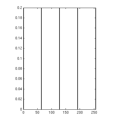
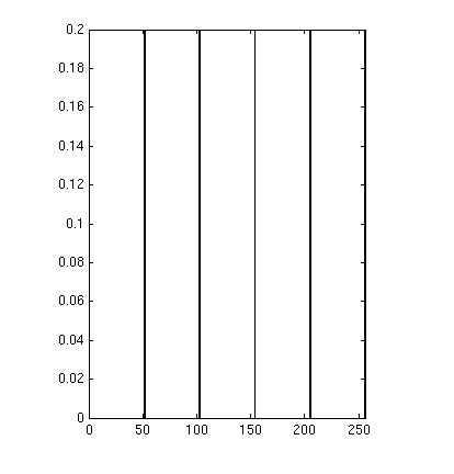
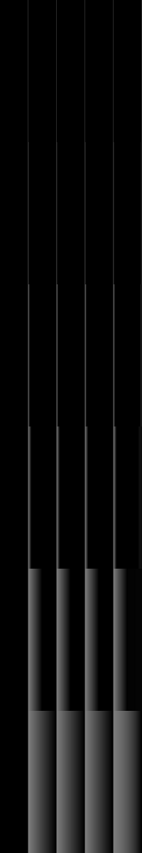
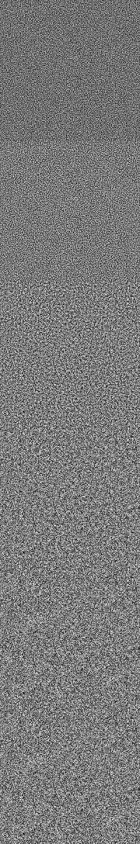
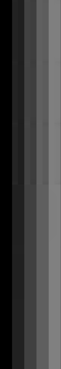
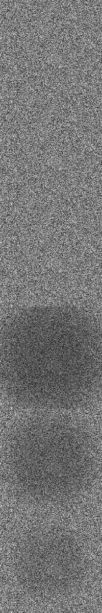
Here are the three images I chose. The first shows bands of
extremely high contrast (as these will be interesting with the later
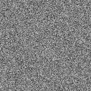
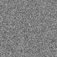
algorithms. The second is pure noise. And the third is an image I
forced into an ugly gray range of a small range of intensities.
|
|
|
|
|
0.0795 s |
|
|
|
|
|
0.0300 s |
|
|
|
|
|
0.0810 s |
As expected
from the bands, the result doesn't seem to modify them much. It
changes the values slightly due to the nature of the algorithm, but
we still get bands of relatively the same color. With the noise we
see little change, as expected, this histogram is nearly already
flat. Something interesting to note is in the right histogram.
Because a few intensities DO get shifted, and because it already is
mostly flat, we get a few peaks that are nearly twice as tall as the
original image. Visually it doesn't make a difference, but for an
almost flag image, histogram equalization can have such
artifacts. And lastly, with Wall-E we see what we expect to.
Part
6:
Histogram equalization seems highly effective for each of these
images except the two special cases (the bands and the noise). We do
notice here though that histogram equalization gives a sort of night
vision effect. The images are easier to see, but due to scaling some
things appear less realistic. We notice in the Wall-E picture that
there's large jumps between two values which give it a noisy
appearance in the background. While histogram equalization performs
well, this should be taken into consideration when applying it.
Part 7:
To
improve contrast without giving it that almost surreal feel to the
pictures we can blend the two algorithms. The process can be seen
from the images below. I decided to use the crowd image since the
result seemed a little washed out to me. We get the following. The
alpha values were 0.2, 0.4, 0.6, 0.8 (0.0 meaning no change to
original, 1.0 meaning exactly like histogram equalization.
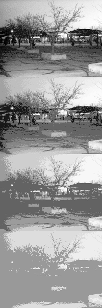
I also did a special case to show how important binning is. I used the outside example to show the effect of using less bins. The bin sizes were: 128, 64, 32, 16
Adaptive
Histogram Equalization
Matlab
Function: AHE.m
Part
1:
My implemented version of AHE can be found in AHE.m.
For the approach I decided to use the pixel by pixel approach. I knew
the results would have more artifacts than the tiling approach but I
figured the general implementation would be easier. I did my best to
be smart about decisions made to bring the overall running time down.
When a window size isn't supplied I create one that is about 20% of
the image. This makes for long runs, but gives nicer results than
much smaller windows.
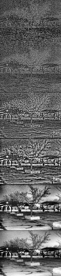
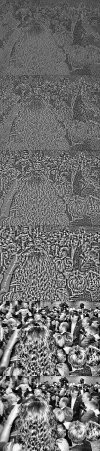
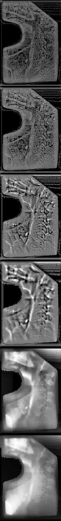
Part 2:
The
window sizes for the below images are: [3 6 12 24 99 198]. Due to
scaling the lowest values look a bit like noise. But in the full
version when zooming in you definitely get crisp lines and shapes.
(Note, I only uploaded the scaled versions for size reasons, to get
the full versions and zoom on them, please run the test file). This
goes to show how crucial different window sizes are.
|
|
|
|
|
|
|
|
|
|
Part 3 &
4:
We can see from the above that the smaller our window size the
more we are effected by changes in our neighborhood. Two interesting
examples here are the bands example and the salt and pepper example.
We can easily see the size of window increasing in the amount of
change in our images. Because it is only effected by changes in it's
neighborhood each of the bands turns to be the same color. Since the
contrast between each of the edges is exactly the same (the values go
0.0, 0.25, 0.50, 0.75, 1.0 so the change between intensities is
always 0.25). In the salt and pepper case it seems to make the image
feel less random. This makes sense, because with small enough window
sizes even the small areas of near consistent (but random)
intensities will be broken apart. In the end we get a still random,
but more uniform image. We note one big limitation of this approach
which is easily seen in the portal example. We notice bands and
chunks where we can definitely see where our window was. The plus
here is that we can see some definite structures (visually) that were
couldn't see before. At a first glance, this may not look as visually
pleasing as straight histogram equalization, but it does bring out
different structures. For instance the shadows on the ladies arm, and
on the wall behind the people in chang are much more crisp. This
makes sense why it is an effective technique for images such as the
portal image.
Part 3:
The
below table shows the time to run AHE with each window size on each
image. All the times are expressed in seconds. The below confirms are
belief that doing the non-tile approach is O(N*M), where N is the
size (N=H*W) of our image and M is the size of our window. (This is
obtained since we have to iterate over the pixels, and recalculate
the histogram which we do in a smart way which requires is only 2*M).
|
|
3 pixels |
6 pixels |
12 pixels |
24 pixels |
99 pixels |
198 pixels |
|
University |
0.23 |
0.26 |
0.37 |
0.59 |
1.74 |
3.01 |
|
Crowd |
0.5 |
0.58 |
0.81 |
1.29 |
3.94 |
7.14 |
|
Chang |
0.97 |
1.12 |
1.56 |
2.46 |
7.38 |
13.3 |
|
Portal |
0.24 |
0.27 |
0.35 |
0.52 |
1.44 |
2.53 |
|
Bands |
0.64 |
0.72 |
0.94 |
1.4 |
4.07 |
7.22 |
|
Salt and Pepper |
0.25 |
0.28 |
0.38 |
0.57 |
1.7 |
2.92 |
We
expect the first column to be somewhere around 3 times slower than
the regular histogram speeds. Indeed as we seem to range from about
2-4 times slower. This agrees with our projected running time.
Clipped
Local Adaptive Histogram Equalization
Function: CLAHE.m
|
|
|
|
|
|
|
|
|
|
CLAHE has the result of decreasing the rate of change heavily.
This shows up visually as a smoothing effect applied to the images.
We see this very easily in the sky of the university image. We see
with the lower threshold the sky is very smooth and clear. As our
threshold gets larger we notice the artifacts in the sky begin to
come back. (This is also easily noticed in the portal images). The
side effect here is that since the image is discouraged from changing
dramatically, it is harder to notice parts of the image that do
change drastically. We can see this on the chang picture as the
shadows on various objects on the table begin to come less and less
sharp.
The bands example now looks fairly neat. Since it's not allowing us to focus too largely on the areas of change now, we start to see them as distinct bands again. With a small enough threshold we get a shading effect around the borders. We also see in the salt and pepper example that as the window gets larger we start to get more histograms that are clipped. And by clipping and spreading that value throughout the rest of the histogram, we begin to get a gray haze around the image. It discourages the heavy change, the very nature of the salt and pepper image. This explains why the lower images are generally darker, because we're spreading clipped values back into the mass of the image. One drawback we see from the noise is that since we use a hard threshold value we get a spherical haze. This happens since there are less values to add to our histogram near the edges. Having more values to add to the histogram gives us a greater chance of clipping. This later helped me realize that perhaps instead of converting the percentage passed in into a hard threshold we could calculate the threshold on the fly. I didn't do this, but it wouldn't be that hard to do.
Note: My CLAHE approach copies most of the code from my AHE approach, but modifies a small portion to add the CL to CLAHE.