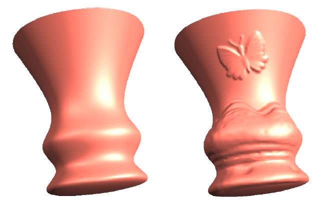
Copy and Paste Editing of Multi-resolution Surfaces

Vase

Example of pasting from the Biermann paper.

Abe Stephens and Won-Ki Jeong
CS-6620 Final Project Spring 2004.
(c) 2004 Scientific Computing and Imaging Institute
Salt Lake City.

Based on the papers:
Cut-and-Paste Editing of Multiresolution Subdivision Surfaces. Henning Biermann, Ioana Martin, Fausto Bernardini, Denis Zorin. ACM Transactions on Graphics, vol 21, Number 3, Proceedings of ACM Siggraph, pages 312-321, July 2002. (PDF)
Least Squares Conformal Maps for Automatic Texture Atlas Generation. Bruno Lévy, Sylvain Petitjean, Nicolas Ray, Jerome Maillot. ACM Transactions on Graphics, vol 21, Number 3, Proceedings of ACM Siggraph, Pages: 362 - 371 July 2002. (PDF)

Introduction

This project implements cut-and-paste editing of surfaces. Both the input and output mesh are multiresolution subdivision surfaces that are defined as a base mesh with detail offsets. After the user specifies regions to cut and to paste, the base and detail surfaces on both source and target surfaces are split and base surfaces are parameterized into a common domain.Detail offsets from the source detail surface are copied and transferred to the target surface.
This project resembles a boxed set of recent SIGGRAPH achievements. The basis of the mesh data structure is from Interactive Multiresolution Mesh Editing by Zorin et al (SIG '97), which proposed multiresolution subdivision surface based on Loop subdivision and Laplacian smoothing. Parameterization, one of the most active research fields, is the main technique used for copying details from one surface to the other. Here we are borrowing a subset of the techniques presented in Least Squares Conformal Maps for Automatic Texture Atlas Generation, Levy et. al. (SIG'02). Implementing least-squares subdivision surface fitting and calculating geodesic distance on the surface is also required.
The motivation for choosing this project is that it would be one of the useful extension of what we have done in the class. We have implemented half-edge mesh class, simplification algorithm, and subdivision algorithm- which can be extended to multiresolution mesh structure with reasonable efforts. In addition, cut-and-pasting editing on triangle meshes would not only be intersting but also be useful for the future research.

Implementation

Multi-Resolution Mesh Data Structure

Our multiresolution mesh is based on a half-edge triangle mesh data structure and Loop subdivision. For each subdivision level, newly created vertices, faces, and edges are stored along with detail vectors captured with respect to a local coordinate frame defined on each vertex. Switching between levels either validates or invalidates triangles, edges, or vertices. Since triangles and edges from different levels do not overlap, adjacent information stored in them can be preserved. However, the adjacent edge for each vertex is changed between different level because the vertices from lower levels may be used in the higher ones. This requires storing additional adjacent edge information for each vertex.

The multi-resolution analysis operation is performed by downsampling the mesh and sampling detail vectors. As in Zorin et al (SIG '97), we use Taubin's non-shrinking Laplacian smoothing as a pseudo inverse of Loop subdivision. Downsampling performs Laplacian smoothing, and detail vectors are captured as difference between the current mesh and subdivided downsampled mesh.

Downsampling : M^k-1 = smooth(M^k)
Detail Sampling : D(M^k) = F^t(M^k-subd(M^(k-1))
(M^k : level k mesh, D(M) : detail vector for mesh M, F^t : inverse of local transformation)

Because adjacent edge of each vertex is stored explicitly the local coordinate frame is calculated by adjacent edge e, vertex normal n, and cross product of e and n. The synthesis operation is simply to subdivide and add detail vectors. Currently adaptive analysis or synthesis is not supported.

Parameterization

Parameterization of both the source and target surfaces was implemented using the least squares conformal map technique from (2). Selecting a region to parameterize and normalizing the size of the parameterization ended up being two unforseen challenges in the implementation, performing the parameterization was very straight forward. Region selection was acomplished by allowing the user to click a series of verticies on the surface of the source mesh. These verticies are connected using Dijkstra's algorithm to find the shortest path between each selected pair. This method is somewhat unpredictable, we used total edge length as a metric in the shortest path algorthm, as a result often the user would be suprised after selecting two verticies and finding that the shortest path of edges did not follow their intended path.
The original author's multiresolution data structure allowed them to quickly match the resolution of the source and target meshes. Our implementation used subdivision to compute detail vectors on the source surface but we did not implement any facility for matching the resolution of the source and target surfaces. This resulted in aliasing problems when sampling detail from a fine mesh on to a coarse one.

Geodesic Walking

Once a user selects a source region, the corresponding target region has to be found. We use "Geodesic Walking" to find a region on the target surface. The selected source region is parameterized into a 2D domain, and the center of the region in 2D can be found by the average of boundary vertices of that region. We can connect the center to every vertex on the region boundary to make a set of line segments, and each line segment can be parameterized by the angle from the previous line segment (0 for the first line segment) and the distance from the center. Then we can find a corresponding curves on on the target surface by walking on the surface along the direction and the distance. Distances measured on the parameter domain are relative distances, which means we can zoom in/out on the target surface by uniformly scaling the distances on the 3D.

To map a line segment on 2D parameter space to a curve on the 3D target surface, we need a way to walk on the surface along the given direction with the distance. Once a start point and a direction is given, then we find a surface normal on the point and build a plane that encloses the point, normal vector, and the direction vector. Then we find the intersection between the plane and the surface until its length reaches the given value (distance). Since our mesh is piecewise-linear triangular mesh, we approximate plane-surface intersection by plane-triangle intersection. For each intersected triangle, a starting point is given on the edge, and its surface normal is approximated by the average of the end vertex normals of that edge. Then the curve on the surface is approximated by the set of line segments, and the distance of the curve is the sum of the length of each line segment. Once the target region is found, then it is parameterized onto the common domain where source region is parameterized, and surface detail is transferred between two meshes.

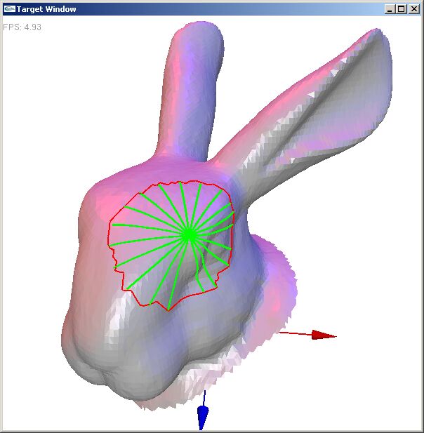
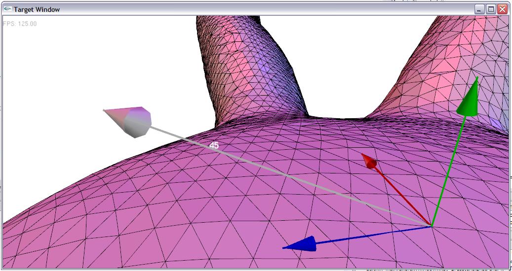
Fig. Target region selection by Geodesic walking on the surface

Detail Transfer

Transfering detail vectors from the source to the target surface is the final stage in the copy and paste process. It consists of the three following steps:

Intersect target verticies with source faces.
Linearly interpolate the source detail vectors with the position of each intersected target vertex.
Move the interpolated source detail vector to the target surface.

Vertex and face intersection of the 2D parameterized meshes was implemented using a brute force query. This was acceptable since the size and resolution of the selected areas was very small. For each vertex of the target surface, the three verticies of the source triangle which contained that vertex were interpolated. Since the detail vector of each vertex on the source surface was defined using an independent coordinate, the three detail vector needed to be transformed to a common world coordinate system before they could be iterpolated. The target vertex detail vector is replaced by the result of transforming and interpolation the source detail vectors. There are five different coordinate frames involved in detail transfer, three transformations and an interpolation, each source vertex has its own frame which is transformed into the world coordinate frame for interpolation, and the interpolated detail vector is placed in the coordinate frame of the target vertex.
Our formulation allowed each vertex to use an independent coordinate frame that was computed as a function of the normal at a given point and a global orientation rule. Given the location of the vertex and its normal, a plane was computed, and the orientation vector was projected to the plane. The direction of this projected point formed the second axis of the local coordinate system, in the case that the global orientation vector was tangent to the plane, a second orientation was used. Since the same rules were used to find the local coordinate frames of each vertex during sampling and detail transfer, the displacement vector remained consisted between the two stages of the algorithm. Maintaining this consistency was the last bug encountered before the expected output was produced.

Screen Shots

Work in progress: Selecting a region and computing parameterization.

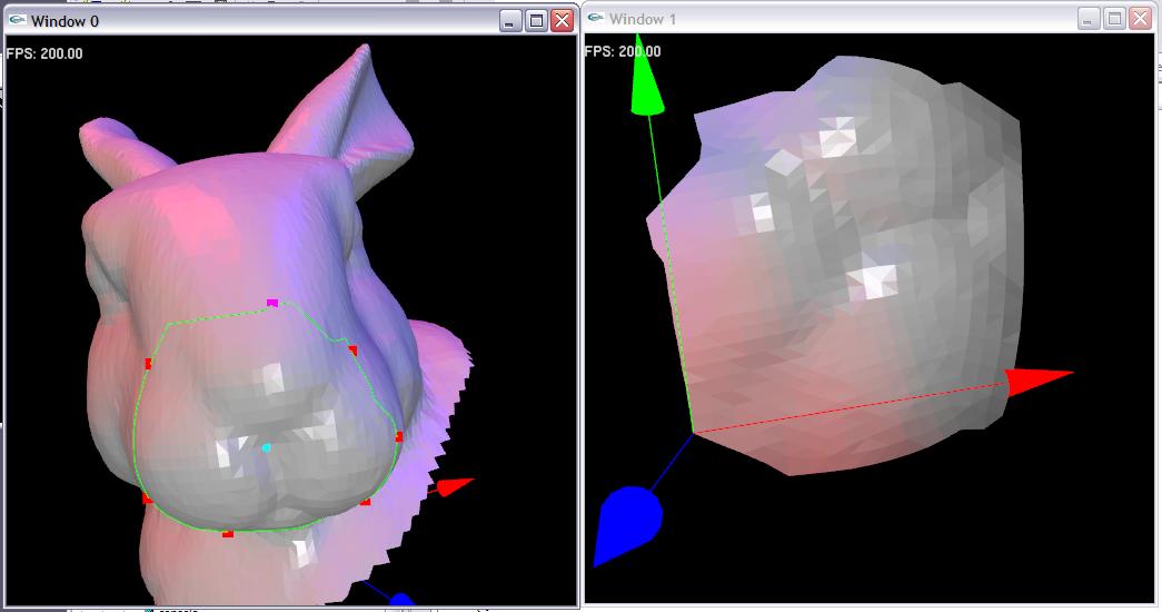
Building a widget for target region selection and orientation.

Early output problems.

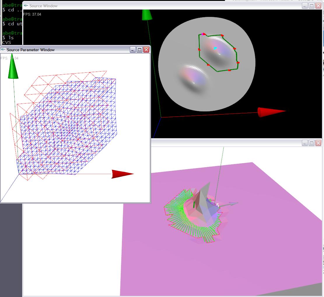
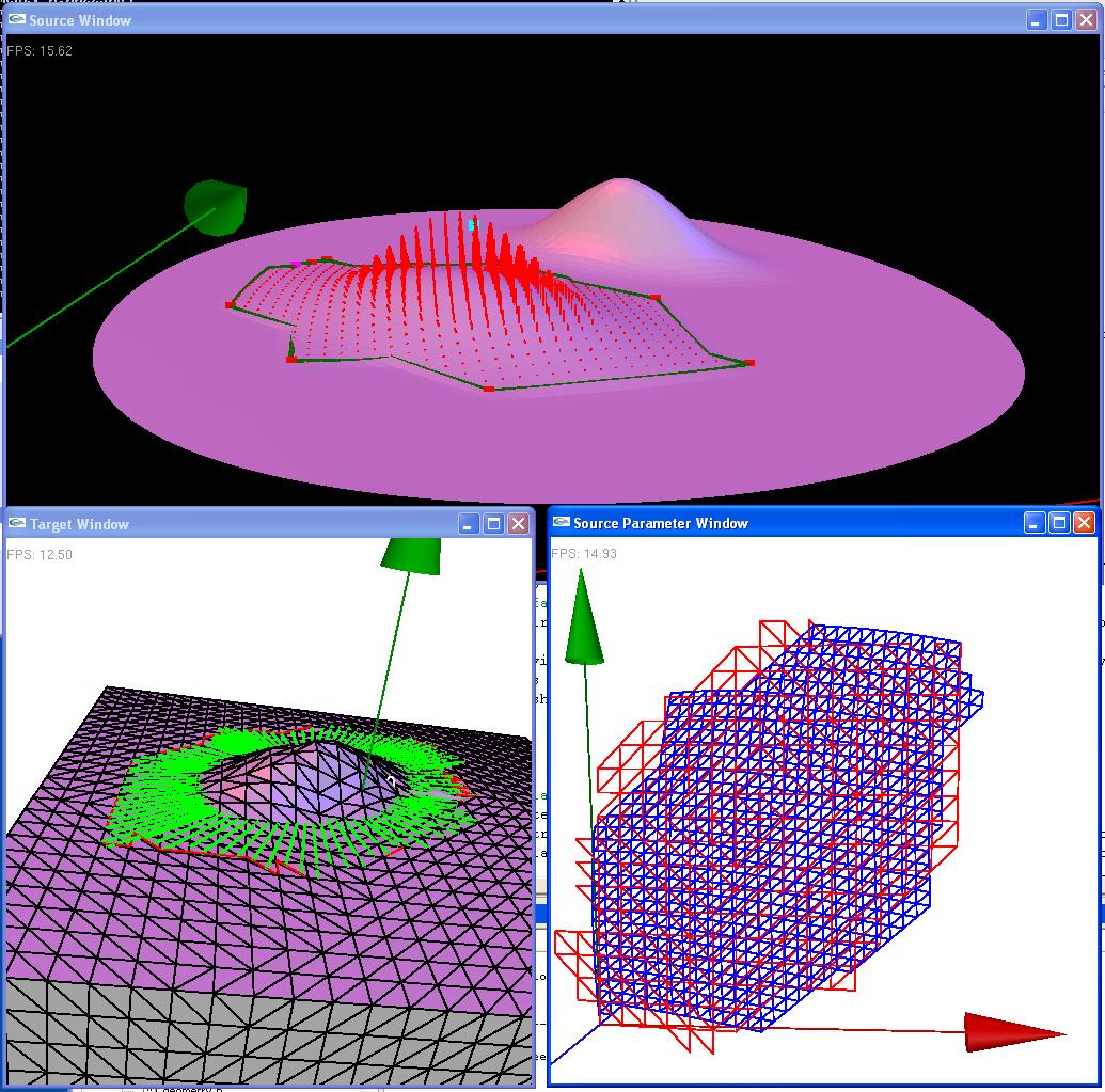
Local frame for computing displacement vectors of source verticies is different then the local frame that displacement is interpolated in.

Final output. The red vectors in the upper window indicate the sampled detail vectors.

Usage:

Set source and target mesh variables and load commands in editmm_window0.txt and editmm_window2.txt.
Execute the program.
Press 't' on the Source window.
Click a border on the source mesh. Take care that the border does not self intersect.
Click the center of the selected region.
Issue "base" command.
Press '>' or '<' to build base detail vectors.
Press 'n' when finished.
Issue "param"
Move the Source Param window to view the result.
Press 'w' in the source param window to enable wireframe.
Issue "target" in the target window.
Click the target mesh and select a point.
Use '<' '>' '-' and '+' to orientate and scale the target region selection.
Press 'd' when finished.
Issue Param <targetfile.m>
View result in Parameter window.
Issue "detail" in target window.

Total project size was 23999 lines of code.